Visual Dashboard: Performing Statistical Analyses with Visual Tools
Visual Dashboard
Analysis Gadgets
Chart
Analysis Gadget Charts
Visual Dashboard produces histograms, scatter plots, pie charts, and bar and line graphs directly from data files. This option produces charts based on the types of data available in the project. The Chart option is capable of generating the following chart types:
- Column charts use vertical bars to represent the count or weight for each value of the main variable(s). Each series results in an additional vertical bar at each point.
- Line charts connect X and Y data points with straight lines. Each series is represented by a different style of line and both variables must be numeric.
- Area charts lay series on top of one another for comparison purposes and can be used to illustrate volume as well as counts.
- Pie charts use a circle to represent each series and each value of the main variable has a slice of the circle proportional to the value associated with it.
- Aberration detection charts use line charts to monitor changes in the distribution or frequency of health events when compared to historical data.
- Pareto charts use vertical bars to represent the count or weight for each value of the main variable(s) and a dashed line to represent the accumulated percentage. Each series results in an additional vertical bar at each point.
- Scatter charts display variables along an X-Y axis as a scatter plot. The X variable is the independent variable and Y variable is the dependent variable. Each series is represented by a different point style.
- Epi Curve charts use vertical bars to represent the count or weight for each value of the main variable. Each series creates an additional vertical bar at each point. The main variable must be either numeric or date/time. This graph differs from the bar graph because adjacent bars represent equal ranges of the main variable.
The examples below demonstrate how to create each of the charts.
Column Chart
Follow the steps below to create a bar graph using data from the Sample.PRJ project.
- Open the Sample.PRJ project and select the Oswego form.
- Right click on the canvas and select Add Analysis Gadget > Charts > Column chart. The Column Chart gadget configuration window opens to the Variables property panel.
- From the Main variable drop-down list, select the variable Age to use for the independent variable.
- Leave the Weight and One graph for each value of option at the default setting (none).
- Click OK. The graph appears on the canvas, displaying in columns the number of patients by age.

Figure 8.43: Column chart
Line Chart
Follow the steps below to create a line chart showing counts by date of onset of illness.
- Open the EColi.PRJ project and select the Food History form.
- Right click on the canvas and select Add Analysis Gadget > Charts > Line chart. The Line Chart gadget configuration window opens to the Variables property panel.
- Select Onset Date from the Main variables list.
- The system returns a line chart of onset dates between April and May from the dataset.
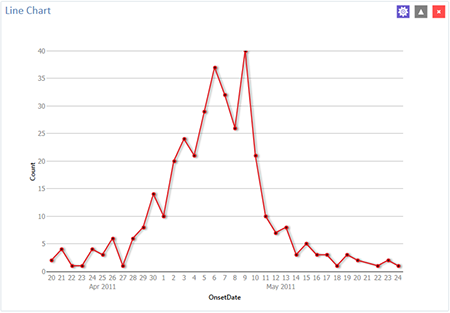
Figure 8.44: Line chart
Area Chart
Follow the steps below to create an area chart showing fever temperatures of church supper attendees.
- Open the EColi.PRJ project and select the Food History form.
- Right click on the canvas and select Add Analysis Gadget > Charts > Area chart. The Area Chart gadget configuration window opens to the Variables property panel.
- Select OnsetDate from the Main variables list.
- The system returns a line chart of onset dates between April and May from the dataset.
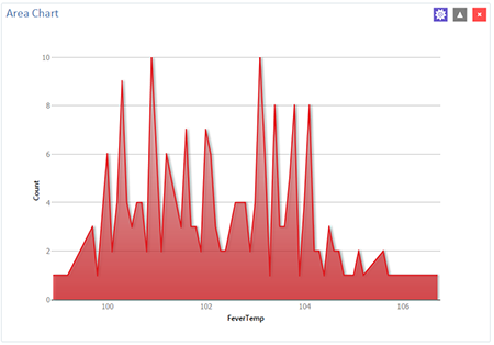
Figure 8.45: Area chart
Pie Chart
Follow the steps below to create a pie chart showing age groups of church supper attendees. The dataset has individual ages. To create age groups, you can define a new variable with recoded values making age groups from age 0 to age 70 grouped by 10 years per group. Detailed instructions about how to use the Defined Variables gadget are in the Create a New Variable section later in this guide.
- Open the Sample.PRJ project and select the Oswego form.
Recode the Age variable using the Defined Variables gadget.- On the left-hand side of the Visual Dashboard canvas, move the mouse cursor over the Defined Variables gadget. The gadget expands and becomes fully visible.
- Click the New Variable button.
- Select With Recoded Value. The Add Recoded Variable dialog box appears.
- From the Source field drop-down list, select Age. Notice the Destination field is populated with Age_RECODED.
- Click the Fill Ranges button. The Fill Ranges dialog box appears.
- Enter 0 for Start value, 70 for End value, and 10 for By.
- Click OK. The From, To, and Representation columns populate within the Add Recoded Variable window.
- Click OK. The variables are recoded and are listed in the Defined Variables gadget window.
- Right click on the canvas and select Add Analysis Gadget > Charts > Pie chart. The Pie Chart gadget configuration window opens to the Variables property panel.
- From the Main variable drop-down list, select the variable AGE_RECODED.
- Leave the Weight and One graph for each value of option at the default setting (none).
- Click OK. The graph appears on the canvas.

Figure 8.46: Pie chart
The chart shows the age groups of church supper attendees.
Aberration Detection
The Aberration Detection Analysis gadget can be used with syndromic or national surveillance data. It is designed to monitor changes in the distribution or frequency of health events when compared to historical data. This gadget uses an algorithm implemented by the Early Aberration Reporting System (EARS), which is a tool developed by CDC’s Division of Bioterrorism Preparedness and Response to assist local-level health offices with early detection of bioterrorism events or possible outbreaks.
The example described here uses an Excel spreadsheet named EARS.xls that comes with Epi Info™ 7 and is located in the ProjectsSample project folder.
- Right click on the canvas and choose “Set data source,” or click the data source icon in the toolbar to Select Data Source.
- Click the Database Type drop-down to select Microsoft Excel 97-2003.
- Click Browse and then Browse again to browse for the EARS.xls file.
- Browse to the Epi Info 7ProjectsSample folder and select the EARS.xls file.
- Click on Sheet 1$, then click OK.
- Right click on the canvas and select Add Analysis Gadget. Scroll to highlight Charts, then select Aberration Detection. The Aberration Detection gadget configuration window opens to the Variables property panel.
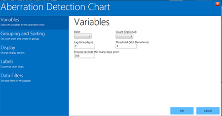
Figure 8.47: Aberration Detection gadget
- From the Date drop-down list, select the variable, DATE.
- From the Count (Optional) drop-down list, select the variable, COUNT. Leave the default settings for Lag Time, Threshold, and Process Records This Many Days Prior.
- Click Grouping and Sorting to that property panel.
- From the Indicators list, click the variable SYNDROME.
- Click OK. The Aberration Detection line graph displays on the canvas.

Figure 8.48: Aberration Detection line graph
The chart and table display aberrations found, date, count, expected count, and the standard deviations. The current number of patient visits with Asthma is higher (Count: 66) than the defined threshold (Expected; 20.57), hence the aberration detected on 12/05/2010. Aberrations may need to be evaluated by an epidemiologist (or other public health professional) to determine whether they signify an event of public health importance warranting further investigation.
Pareto Chart
Follow the steps below to create a Pareto chart showing age groups of church supper attendees. The dataset has individual ages. To create age groups, you can define a new variable with recoded values making age groups from age 0 to age 70 grouped by 2 years per group. Detailed instructions about how to use the Defined Variables gadget are in the Create a New Variable section later in this guide.
- Open the Ecoli.PRJ project and select the FoodHistory form.
- Recode the Age variable using the Defined Variables gadget.
- On the left-hand side of the Visual Dashboard canvas, move the mouse cursor over the Defined Variables gadget. The gadget expands and becomes fully visible.
- Click the New Variable button.
- Select With Recoded Value. The Add Recoded Variable dialog box appears.
- From the Source field drop-down list, select Age. Notice the Destination field is populated with Age_RECODED.
- Click the Fill Ranges button. The Fill Ranges dialog box appears.
- Enter 0 for Start value, 70 for End value, and 2 for By.
- Click OK. The Add Recoded Variable window appears with the From, To, and Representation columns populated.
- Click OK.
- Right click on the canvas and select Add Analysis Gadget > Charts > Pareto chart. The Pareto Chart gadget configuration window opens to the Variables property panel.
- From the Main variable drop-down list, select the new variable, Age_RECODED.
- Click the Labels option to customize chart labels and axes.
- Update the X-axis angle setting to -90. This step will permit the date values to display fully on the X-axis.
- Click the Display option.
- Change the width setting to 1000. If your computer screen is too small, you might need to change the width setting of the chart to a higher number until the system displays the X-axis labels.
- Click OK. The Pareto chart appears on the canvas.
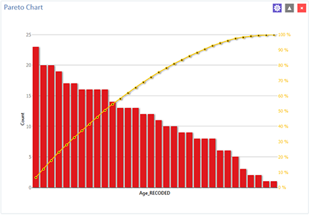
Figure 8.49: Pareto chart
Scatter Chart
Follow the steps below to create a scatter XY graph using data from the Sample.prj project.
- Open the Sample.PRJ project and select the EstriolAndBirthweight form.
- Right click on the canvas and select Add Analysis Gadget > Charts > Scatter chart. The Scatter Chart gadget configuration window opens to the Variables property panel.
- From the Main variable drop-down list, select the variable Estriol to use for the independent variable.
- From the Outcome variable drop-down list, select the variable Birthweight to use for the independent variable.
- Click OK. The graph appears on the canvas, displaying the scatter plot of data points showing the level of Estriol along the X-axis by Birthweight along the Y-axis. A line representing the Linear Regression of the two variables is also included on the chart.
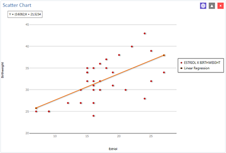
Figure 8.50: Scatter chart
Epi Curve
Follow the steps below to create an Epi Curve showing the incubation time for an unknown pathogen.
- Open the Ecoli.PRJ project and select the FoodHistory form.
- Right click on the canvas and select Add Analysis Gadget > Chart > Epi curve chart. The Epi Curve Chart gadget configuration window opens to the Variables property panel.
- From the Main variable drop-down list, select OnsetDate.
- Click the Labels option to customize chart labels and axes.
- Update the X-axis angle setting to -90. This step will permit the date values to display fully on the X-axis.
- Click the Display button. The Display property panel appears.
- Change the width setting to 1000. If your computer screen is too small, you might need to change the width setting of the chart to a higher number until the system displays the values.
- Click the Legend button. The Legend property panel appears.
- Click the checkmark to select Show Legend.
- Click the Grouping and Sorting button. The Grouping and Sorting property panels appears.
- In the Stratify by: list, scroll down and select the variable Sex.
- Click OK. The Epi Curve chart appears on the canvas. Note that hovering over any bar on the chart will display the date and count for the associated data series.
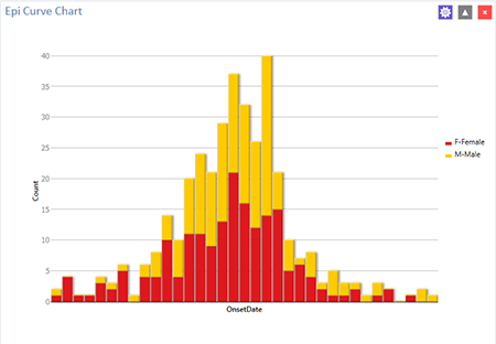
Figure 8.51: Epi Curve chart