Classic Analysis: Command Driven Analyses and Data Management
‹View Table of Contents
How to Use Advanced Statistics
Use the REGRESS Command
The REGRESS command performs linear regression and contains support for automatic dummy variables and multiple interactions.
REGRESS can be used for simple linear regression (only one independent variable), for multiple linear regression (more than one independent variable), and for quantifying the relationship between two continuous variables (correlation). Regression is used when you want to predict one dependent variable from one or more independent variables.
Syntax
REGRESS <dependent variable> = <independent variable(s)> [NOINTERCEPT] [OUTTABLE=<tablename>] [WEIGHTVAR=<weight variable>] [PVALUE=<PValue>]
Dialog Box

Figure 9.62: Linear Regression Window
- The Outcome Variable is the dependent variable for the regression.
- Other Variables appear in the predictor variables list.
- Interaction Terms are defined with the Make Interaction button. Make Interaction appears if two or more variables are selected from the Other Variables list box. If you click Make Interaction, the relationship populates the Interaction Terms list box.
- Make Dummy is activated if you select a predictor variable. If you select a numeric variable, it will be treated as discrete rather than continuous; the variable is enclosed in parentheses to indicate that dummy variables are being created. If a predictor variable enclosed in parentheses is selected in the list, the Make Dummy button changes to Make Continuous. Selecting it results in the variable being treated as continuous. If you select more than one predictor variable, the Make Dummy button changes to Make Interaction. Selecting it results in all possible combinations of the selected variables being added to the regression as interaction terms.
- A Weight variable may selected to use in weighted analyses.
- Confidence Limits specifies the probability level at which confidence limits are computed (default=.05).
- The Output to Table field identifies a table to receive output from the command. (Currently Disabled).
- If you select No Intercept, the regression is performed without a constant term, forcing the regression line through the origin.
- OK accepts the current settings and data, and subsequently closes the form or window.
- Save Only saves the created code to the Program Editor, but does not run the code.
- Cancel closes the dialog box without saving or executing a command.
- Clear empties the fields so information can be re-entered.
- Help opens the Help topic associated with the module being used. (Currently Disabled).
How to Use
- From the Analysis Command Tree, use the READ command to open a PRJ project file. Select a form or table.
- From the Analysis Command Tree, click Advanced Statistics > Linear Regression. The REGRESS dialog box opens.
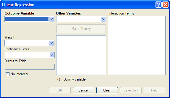
Figure 9.63: Linear Regression Window
- From the Outcome Variable drop-down list, select a variable to be the dependent variable for regression.
- From the Other Variables drop-down list, select the variable(s) to be the predictors.
- If you select any predictor variables, Make Dummy will be activated. Selecting one will allow a numeric variable to become discrete rather than continuous; the variable is enclosed in parentheses to indicate that dummy variables are created. If a predictor variable enclosed in parentheses is selected, the Make Dummy button changes to Make Continuous. Selecting it makes the variable continuous. If you select more than one, the Make Dummy button changes to Make Interaction. Selecting it adds all possible selected combinations to the regression as interaction terms.
- Make Interaction appears if you select two or more variables from the Other Variables list box. Interaction Terms are defined with the Make Interaction button. Click Make Interaction. The relationship populates the Interaction Terms list.
- The Output to Table field identifies a data table to receive output from the command. Results can be sent to an output table for graphing. (Currently Disabled).
- If No Intercept is selected, the regression is performed without a constant term, forcing the regression line through the origin.
- Click OK. Results appear in the Output window.
Try It
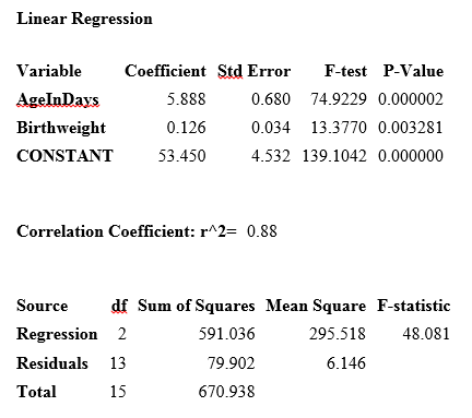
- Read in the project Sample.PRJ. Open BabyBloodPressure.
- Click Linear Regression. The REGRESS dialog box opens.
- From the Outcome Variable drop-down list, select SystolicBlood.
- From the Other Variables drop-down list, select AgeInDays.
- From the Other Variables drop-down list, select Birthweight.
- Click OK. Results appear in the Output window.
Use the LOGISTIC Command
The Logistic Regression command performs conditional or unconditional multivariate logistic regression with automatic dummy variables and support for multiple interactions. The dependent (Outcome) variable must have a Yes/No value. Records with missing values are excluded from the analyses.
Independent (Other Variables) can be numeric, categorical, or Yes/No variables. Missing is interpreted as missing, 0 is false, and any other response is true. Independent variables are controlled by the Include Missing setting. If Include Missing is used with missing values and true and false, dummy variables will be made automatically, which contribute Yes vs. Missing and No vs. Missing. Independent variables of text type are automatically turned into dummy variables, which compare each value relative to the value lowest in the sort order. Date or numeric type Independent variables are treated as continuous variables unless surrounded by parentheses in the command. If that occurs, they automatically turn into dummy variables which compare each value relative to the lowest value.
Syntax
LOGISTIC <dependent variable> = <independent variable(s)> [MATCHVAR=<match variable>] [NOINTERCEPT] [OUTTABLE=<tablename>] [WEIGHTVAR=<weight variable>] [PVALUE=<PValue>]
Dialog Box
- From the Analysis Command Tree, use the READ command to open a PRJ project file. Select a form or table.
- From the Analysis Command Tree, click Advanced Statistics > Logistic Regression. The LOGISTIC dialog box opens.
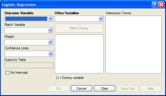
Figure 9.64: Logistic Regression Window
- From the Outcome Variable drop-down list, select a variable to act as the dependent variable for regression.
- From the Other Variables drop-down list, select the variable(s) to act as the predictors.
- If you select any predictor variables, Make Dummy will be activated. Selecting one will allow a numeric variable to become discrete rather than continuous; the variable is enclosed in parentheses to indicate that dummy variables are created. If a predictor variable enclosed in parentheses is selected, the Make Dummy button changes to Make Continuous. Selecting it makes the variable continuous. If you select more than one, the Make Dummy button changes to Make Interaction. Selecting it adds all possible selected combinations to the regression as interaction terms.
- Make Interaction appears if two or more variables are selected from the Other Variables list box. Interaction Terms are defined with the Make Interaction button. Click Make Interaction. The relationship populates the Interaction Terms list.
- Match Variable identifies the variable indicating the group membership of each record.
- The Output to Table field identifies a data table to receive output from the command. Results can be sent to an output table for graphing. (Currently Disabled).
- If No Intercept is selected, the regression is performed without a constant term forcing the regression line through the origin.
- Click OK. Results appear in the Output window.
Try It
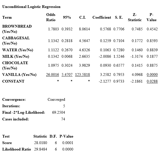
- Read in the project Sample.PRJ. Open Oswego.
- Click Logistic Regression. The LOGISTIC dialog box opens.
- From the Outcome Variable drop-down list, select ILL.
- From the Other Variables drop-down list, select BROWNBREAD, CABBAGESAL, WATER, MILK, CHOCOLATE, and VANILLA.
- Click OK. Results appear in the Output window.
Use the KMSURVIVAL Command
The KMSURVIVAL command performs Kaplan-Meier (KM) Survival Analysis. The objective of this methodology is to estimate the probability of survival of a defined group at a designated time interval. KM uses a non-parametric survival function for a group of patients (their survival probability at time t) and does not make assumptions about the survival distribution.
What distinguishes survival analysis from most other statistical methods is the presence of “censoring” for incomplete observations. In a study following two different treatment regimens, analysis of the trial typically occurred well before all patients died. For those still alive at the time of analysis, the true survival time was known only to be greater than the time observed to date. These observations are called “censored.” Two other sources of incomplete observation are patients “lost to follow-up,” and the appearance of an event other than the event being studied.
Survival analysis requires censored and time variables, the units of time, and the groups being compared.
Syntax
KMSURVIVAL <TimeVar> = <GroupVar> * <CensorVar> (<Value>) [TIMEUNIT="<TimeUnit>"] [OUTTABLE=<TableName>] [GRAPHTYPE ="<GraphType>"] [WEIGHTVAR=<WeightVar>]
Dialog Box
- From the Analysis Command Tree, use the READ command to open a PRJ project file. Select a form or table.
- From the Analysis Command Tree, click Advanced Statistics > Kaplan-Meier Survival. The Kaplan-Meier Survival dialog box opens.
- From the Censored Variable drop-down list, select the variable that indicates whether the case is a failure or a censored case.
- From the Value for Uncensored drop-down list, select the value of the censored variable that indicates a failure.
- From the Time Variable drop-down list, select the variable that indicates at which time the failure or censorship occurred.
- From the Test Group Variable drop-down list, select the discrete variable used to divide cases into groups.
- Click OK. Results appear in the Output window.
- A Survival Probability graph is produced by default. Use the Graph Type drop-down list to select the Log-Survival graph type or None to view the results in a table.
Try It
- Read in the Sample.PRJ project. Check the checkbox to Show Tables and scroll down to open the Addicts table.
- Click KAPLAN-MEIER SURVIVAL. The Kaplan-Meier Survival dialog box opens.
- From the Censored Variable drop-down list, select Status.
- From the Value for Uncensored drop-down list, select 1.
- From the Time Variable drop-down list, select Survival_Time_Days.
- From the Test Group Variable drop-down list, select Clinic.
- Click OK. Results appear in the Output window.
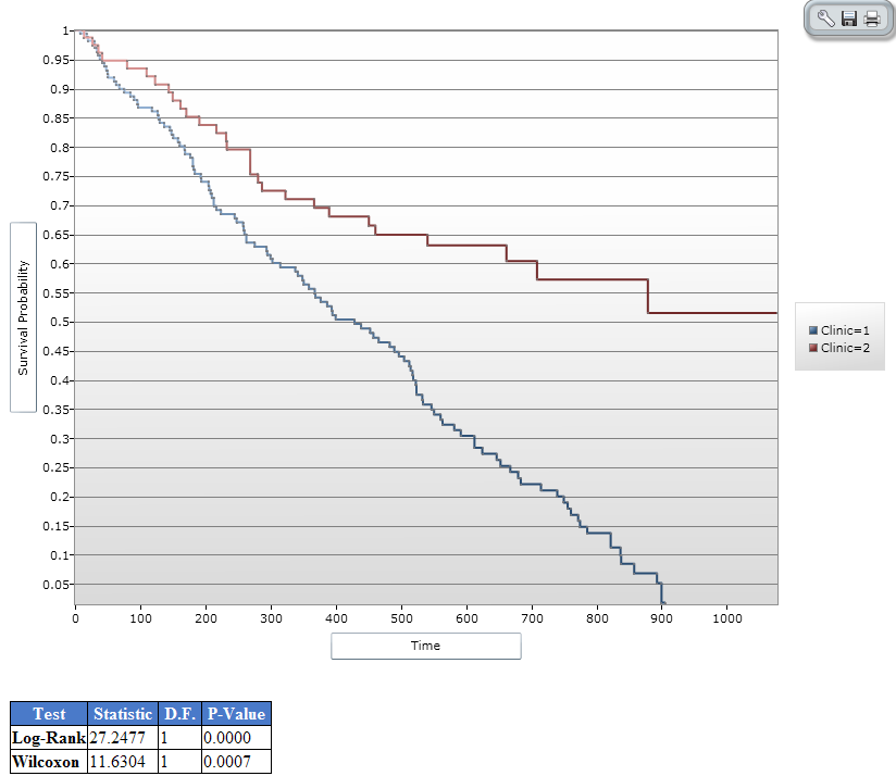
Figure 9.65: Results of Kaplan-Meier Example Survey
Use the COXPH Command
The COXPH command performs Cox Proportional Hazards survival analysis. This form of survival analysis relates covariates to failure through hazard ratios. A covariate with a hazard ratio less than one suggests improved survival for the level being compared with the reference level. COXPH output includes regression coefficients, test statistics with p-values, hazard ratios, and cumulative survival plots.
What distinguishes survival analysis from most other statistical methods is the presence of “censoring” for incomplete observations. In a study following two different treatment regimens, analysis of the trial typically occurred well before all patients died. For those still alive at the time of analysis, the true survival time is known only to be greater than the time observed to date. These observations are called “censored”. Two other sources of incomplete observation are patients “lost to follow-up”, and the appearance of an event other than the event being studied.
Survival analysis requires censored and time variables, the units of time, and the groups being compared.
Syntax
COXPH <time variable>= <covariate(s)>[: <time function>:] * <censor variable> (<value>) [TIMEUNIT="<time unit>"] [OUTTABLE=<tablename>] [GRAPHTYPE="<graph type>"] [WEIGHTVAR=<weight variable>] [STRATAVAR=<strata variable(s)>] [GRAPH=<graph variable(s)>]
Dialog Box
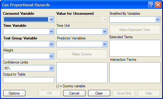
Figure 9.66: Cox Proportional Hazards Dialog Box
- The Censored Variable indicates whether the case is a failure or censored.
- The Time Variable indicates at which time the failure or censorship occurred.
- Test Group Variable is a discrete variable used to divide cases into groups for comparison. In the Cox model, there is no essential difference between the group variable and other predictor terms. For this reason, its use is optional.
- A Weight variable is selected for use in weighted analyses. The weight variable applies to all aggregation clauses.
- Confidence Limits indicate the probability level at which confidence limits should be computed (default=.05).
- The Output to Table field identifies a data table to receive output from the command. (Currently Disabled).
- Value for Uncensored is the value of the censored variable that indicates a failure.
- Time Unit is the unit in which the time variable is expressed.
- Predictor Variables populates the predictor variables list.
- If a predictor variable is selected, Make Dummy is active. If selected, a numeric variable is treated as discrete rather than continuous; the variable is enclosed in parentheses to indicate that dummy variables are being created. If you select a predictor variable enclosed in parentheses, the button changes to Make Continuous. Selecting it results in the variable being treated as continuous.
- Stratify by identifies the variable (if any) to be used to stratify data.
- Options opens the graph selection window and allows you to select variables for graphing and graph types.
- OK accepts the current settings and data, and subsequently closes the form or window.
- Save Only saves the created code to the Program Editor, but does not run the code.
- Cancel closes the dialog box without saving or executing a command.
- Clear empties the fields so information can be re-entered.
- Help opens the Help topic associated with the module being used. (Currently Disabled).
Try It
- From the Analysis Command Tree, use the READ command to open a PRJ project file. Select a form or table.
- From the Analysis Command Tree, click Advanced Statistics > Cox Proportional Hazards. The Cox Proportional Hazards dialog box opens.
- From the Censored Variable drop-down list, select the variable that indicates whether the case is a failure or a censored case.
- From the Value for Uncensored drop-down list, select the value of the censored variable that indicates a failure.
- From the Time Variable drop-down list, select the variable that indicates at which time the failure or censorship occurred.
- From the Time Unit drop-down list, select the unit in which the time variable is expressed, if needed.
- From the Test Group Variable drop-down list, select the discrete variable used to divide cases into groups.
- In the Cox model, there is no essential difference between the group variable and other predictor terms. For this reason, using the group variable is optional.
- From the Other Variables drop-down list, select the predictor variables.
- If you select any predictor variables, Make Dummy will be activated. Selecting will allow a numeric variable to become discrete rather than continuous; the variable is enclosed in parentheses to indicate that dummy variables are created. If a predictor variable enclosed in parentheses is selected in the list, the Make Dummy button changes to Make Continuous. Selecting it makes the variable continuous. If you select more than one, the Make Dummy button changes to Make Interaction. Selecting it results in all possible combinations of the selected variables being added to the regression as interaction terms.
- Click Graph Options. The Cox Graph Options dialog box opens.
- From the Plot Variables drop-down list, select a graph type.
- From the list box, select a variable(s) to graph.
- Clear the Customize Graph checkbox.
- Click OK. The Cox Proportional Hazards dialog box opens.
- Click OK. Results appear in the Output window.
Try It
- Read in the Sample.PRJ project. Open the Addicts table.
- Click Cox Proportional Hazards. The Cox Proportional Hazards dialog box opens.
- From the Censored Variable drop-down list, select Status.
- From the Value for Uncensored drop-down list, select 1.
- From the Time Variable drop-down list, select Survival_Time_Days.
- From the Test Group Variable drop-down list, select Clinic.
- From the Predictor Variables drop-down list, select Methadone_dose__mg_day and Prison_Record.
- Click Options. The Cox Graph Options dialog box opens.
- From the Plot Variables drop-down list, select Survival Observed.
- From the list box, select Clinic.
- Clear the Customize Graph checkbox.
- Click OK. The Cox Proportional Hazards dialog box opens.
- Click OK. Results appear in the Output window.
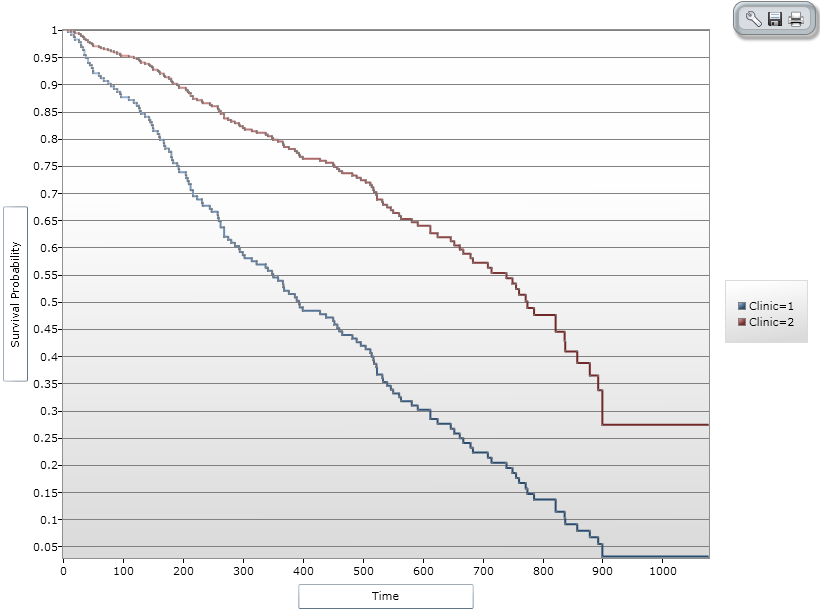
Figure 9.67: Cox Proportional Hazards Graph Result
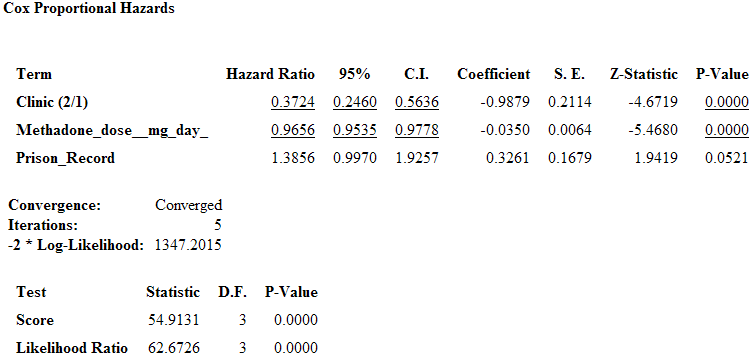
Figure 9.68: Cox Proportional Hazards Statistical Results
Complex Sample Frequencies, Tables, and Means
The Frequencies (FREQ), Tables (TABLES), and Means (MEANS) commands in the Classic Analysis program perform statistical calculations that assume the data comes from simple random (or unbiased systematic) samples. More complicated sampling strategies are used in many survey applications. These may involve sampling features (i.e., stratification, cluster sampling, and the use of unequal sampling fractions). Surveys that include some form of complex sampling include the coverage surveys of the WHO Expanded Program on Immunization (EPI) (Lemeshow and Robinson, 1985) and CDC’s Behavioral Risk Factor Surveillance System (Marks et al., 1985).
The CSAMPLE functions compute proportions or means with standard errors and confidence limits for studies where the data did not come from a simple random sample. If tables with two dimensions are requested, the odds ratio, risk ratio, and risk difference are also calculated.
Data from complex sample designs should be analyzed with methods that account for the sampling design. In the past, easy-to-use programs were not available for analysis of such data. CSAMPLE provides these facilities. It can form the basis of a complete survey system with an understanding of sampling design and analysis.
Complex Sample Frequencies
Dialog Box
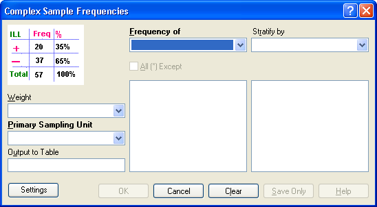
Figure 9.69: Complex Sample Frequencies Dialog Box
- A Weight variable is selected for use in weighted analyses.
- The Output to Table field identifies a data table to receive output from the command.
- Frequency of identifies the variable(s) whose frequency is computed.
- All (*) Except indicates that all the variables except those selected will have frequencies computed.
- Stratify by identifies the variable to be used to stratify or group the frequency data.
- OK accepts the current settings and data, and subsequently closes the form or window.
- Save Only saves the created code to the Program Editor but does not run the code.
- Cancel closes the dialog box without saving or executing a command.
- Clear empties the fields so information can be re-entered.
- Help opens the Help topic associated with the module being used. (Currently Disabled).
Complex Sample Means
Dialog Box
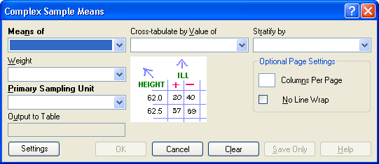
Figure 9.70: Complex Sample Means Dialog Box
- Means of identifies the variable whose mean is to be computed.
- A Weight variable is selected for use in weighted analyses.
- The Output to Table field identifies a data table to receive output from the command. (Currently Disabled).
- Cross-Tabulate by Value of identifies the variable to be used to cross-tabulate the main variable.
- Stratify by identifies the variable to be used to stratify or group the frequency data.
- OK accepts the current settings and data, and subsequently closes the form or window.
- Save Only saves the created code to the Program Editor, but does not run the code.
- Cancel closes the dialog box without saving or executing a command.
- Clear empties the fields so information can be re-entered.
- Help opens the Help topic associated with the module being used. (Currently Disabled).
Complex Sample Tables
Dialog Box
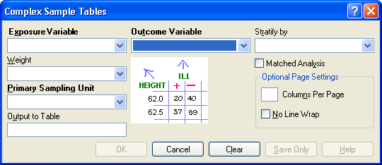
Figure 9.71: Complex Sample Tables Dialog Box
- Exposure Variable identifies the variable that will appear on the horizontal axis of the table. It is considered to be the risk factor (or * for all variables).
- A Weight variable is selected for use in weighted analyses.
- The Output to Table field identifies a data table to receive output from the command.
- Outcome Variable identifies the variable that will appear on the vertical axis of the table.
- Stratify by identifies the variable to be used to stratify or group the frequency data.
- OK accepts the current settings and data, and subsequently closes the form or window.
- Save Only saves the created code to the Program Editor, but does not run the code.
- Cancel closes the dialog box without saving or executing a command.
- Clear empties the fields so information can be re-entered.
- Help opens the Help topic associated with the module being used. (Currently Disabled).