Classic Analysis: Command Driven Analyses and Data Management
‹View Table of Contents
How to Display Statistics and Records
Use the LIST Command
The LIST command creates a line listing of the current dataset. Select specific variables from the Variables drop-down to narrow the list or select * (the Wild Card) to display all the variables. Check the All (*) Except box and select from the Variables drop-down to exclude variables from the list.
To navigate LIST * GRIDTABLE results, use the Tab key to move forward one cell at a time and the Shift+Tab keys to move back one cell at a time. Navigate through the records and cells using the left, right, up, and down arrow keys.
SYNTAX
LIST [<variable(s)>]
LIST *
LIST * EXCEPT [<variable(s)>] {GRIDTABLE}
- From the Classic Analysis Command Tree, use the READ command to open a PRJ project file.
- From the Classic Analysis Command Tree, click Statistics > List. The LIST dialog box opens.
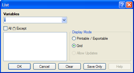
Figure 9.27: List Dialog Box
- Click OK to accept the default settings. The variables in the dataset appear in a grid table inside the Output Window.
- Grid output is not embedded. An Output file is not created.
Create a Web Format List
- From the Classic Analysis Command Tree, click Statistics > List. The LIST dialog box opens.
- From the Display Mode section, select the Printable / Exportable radio button.
- Click OK. The List appears in the Output window in a web table format. Web display mode creates an embedded output file.
Use the FREQ Command
The FREQ command produces a frequency table that shows how many records have a value for each variable, the percentage of the total, and a cumulative percentage. The command FREQ * creates a table for each variable in the current form other than unique identifiers. This command is used to begin analyses on a new data set.
SYNTAX
FREQ <variable(s)>
FREQ *
FREQ * EXCEPT <variable(s)>
- From the Classic Analysis Command Tree, use the READ command to open a PRJ project file.
- From the Classic Analysis Command Tree, click Statistics > Frequencies. The FREQ dialog box opens.
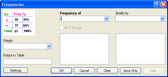
Figure 9.28: Frequency Dialog Box
- From the Frequency of drop-down list, select a variable from the data table.
- Click the All (*) Except checkbox to exclude variables.
- Use the corresponding drop-down lists to select a Weight variable or a Stratify by variable from the data source.
- Use the Output to Table field to specify a location for table results. The new table can be accessed using the READ command.
- Click OK. Results appear in the Output window.
Try It
For this example, use the Classic Analysis Command Tree to generate the FREQ command.
- Read in the Sample.PRJ project. Open Oswego. Seventy five (75) records should be listed in the Output window.
- Click Frequencies. The FREQ dialog opens.
- From the Frequency of drop-down list, select ILL.
- Click OK. Results appear in the Output window.
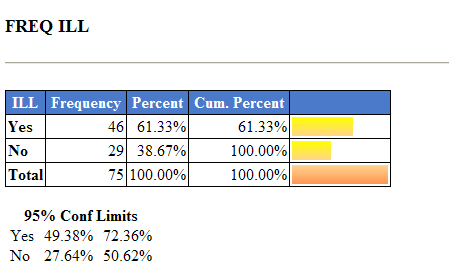
Figure 9.29: Frequency Output Window
- The Frequency column provides the count of individuals that were ill and not ill. The Percent column indicates the percentage of who were ill or not ill.
- The 95% Confidence Limits are a range of values that indicates the likely location of the true value of a measure, meaning (in this instance) that the number of ill could be as low as 49.38%, or as high as 72.36%. Note that the Yes Ill percentage of 61.33% falls within the 95% Confidence Limits range of values based on the data.
Try It
For this example, use the Classic Analysis Command Tree to generate the FREQ command.
- Read in the Sample.PRJ project. Open Oswego. Seventy five (75) records should be listed in the Output window.
- In the Program Editor window, place the cursor under the Read command created. Type FREQ ILL.
- Do not press the Enter key. Leave the cursor on the line of code just created.
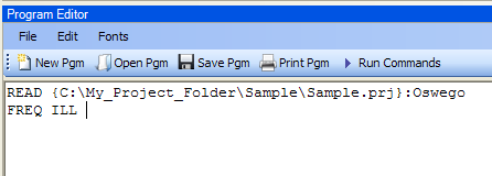
Figure 9.30: Frequency Command in Program Editor
- Click Run Commands from the Program Editor navigation menu. The code turns green indicating syntax review and execution.
- Results of the command appear in the Output window.
- Results are the same as those created using the Command Tree dialog boxes.
Try It
A program or PGM can be saved and run repeatedly against a dataset for continuously updated statistics and analyses.
- Read in the Sample.PRJ project. Open Oswego. Seventy five (75) records should be listed in the Output window.
- Click Open from the Program Editor. The Read Program dialog box opens.
- From the Program drop-down list, select Statistics.
- Click OK. The PGM opens in the Program Editor.
- Click Run. The Program Editor runs the code and output is placed in the Classic Analysis Output window.
- Use the scroll bar to review all the results computed to the Output window.
Use the TABLES Command
The Tables command examines the relationship between two or more categorical values. For 2×2 tables, the Tables command produces odds and risk ratios. A 2×2 table is created when each selected variable has a yes or no answer.
SYNTAX
TABLES <exposure> <outcome> {STRATAVAR=[<variable(s)>]} {WEIGHTVAR=<variable>} {PSUVAR=<variable>} {OUTTABLE=<table>} }
- From the Classic Analysis Command Tree, use the READ command to open a PRJ project file.
- From the Classic Analysis Command Tree, click Statistics > Tables. The TABLES dialog box opens.
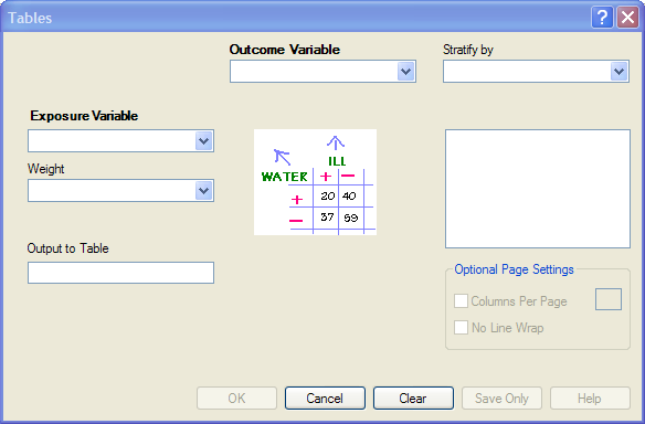
Figure 9.31: Tables Dialog Box
- From the Exposure Variable drop-down list, select a variable from the data to indicate a risk factor exists.
- From the Exposure Variable drop-down list, select a variable from the data to indicate the presence of an outcome. Use the:
- Stratify by drop-down list to select a variable to act as a grouping variable.
- Weight drop-down list to select a variable for weighted Classic Analysis.
- Output to Table field to specify a location for table results.
- READ command to access the READ command.
- Click OK. Results appear in the Output window.
- Scroll down to view the Single Table Classic Analysis.
Try It
Create a 2×2 table using data from the Sample.MDB project.
- Read in the Sample.PRJ project. Open Oswego. Seventy five (75) records should be listed in the Output window.
- Click Tables. The TABLES dialog box opens.
- From the Exposure Variable drop-down list, select Vanilla.
- From the Outcome Variable drop-down list, select ILL.
- Click OK. Results appear in the Output window.
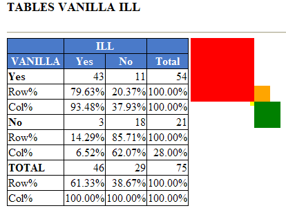
Figure 9.32: Tables Output Window
- Scroll down to view the Single Table Classic Analysis.
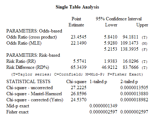
Figure 9.33: Single Tables Classic Analysis
Try It
For this example, use the Classic Analysis Program Editor to create the code.
- Read in the Sample.PRJ project. Open Oswego.
- In the Program Editor window, place the cursor under the Read command created. Type TABLES Chocolate ill.
- Do not press the Enter key. Leave the cursor on the line of code just created.
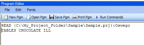
Figure 9.34: Tables Command in Program Editor
- Click Run Commands from the Program Editor navigation menu. The code turns gray indicating syntax review and execution.
- Results of the command appear in the Output window.
- Results are the same as those created using the Command Tree dialog boxes.
Try It
A program or PGM can be saved and run repeatedly against a dataset for continuously updated statistics and analyses.
- To see an example of a PGM, read in the Sample.PRJ project. Open Oswego.
- From the Program Editor, click Open Pgm. The Read Program dialog box opens.
- From the Program drop-down list, select Statistics.
- Click OK. The PGM opens in the Program Editor.
- Click Run Commands. The Program Editor runs the code and output is placed in the Classic Analysis Output window. Use the scroll bar to review all the results computed to the Output window.
Use the MEANS Command
The MEANS command can obtain an average for a continuous numeric variable. Since Yes equals ‘1’ and No equals ‘0’, the mean of a yes-no variable is the proportion of respondents answering yes. For this situation, use the FREQ command. It has two formats. If only one variable is supplied, the program produces a table similar to one produced by FREQUENCIES with descriptive statistics. If two variables are supplied, the first is numeric containing data to be analyzed. The second indicates how groups will be distinguished. The output of this format is a table similar to one produced by TABLES with descriptive statistics of the numeric variable for each group variable value.
SYNTAX
MEANS <variable 1> {<variable 2>} {STRATAVAR=<variable(s)>} {WEIGHTVAR=<variable>} {OUTTABLE=<tablename>}
- From the Classic Analysis Command Tree, use the READ command to open a PRJ project file.
- From the Classic Analysis Command Tree, click Statistics > Means. The MEANS dialog box opens.
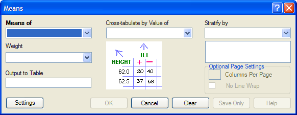
Figure 9.35: Means Dialog Box
- From the Means Of drop-down list, select a variable from the data source.
- The Cross-tabulate by value of drop-down list contains a variable to help determine if the means of a group are equal.
- The Stratify by drop-down list contains a variable to act as a grouping variable.
- The Weight drop-down list contains a variable for weighted Classic Analysis.
- The Output to Table field specifies a location for table results. The new table can be accessed using the READ command.
- Click OK. The Output window populates with the results. Scroll down to view the Mean and Standard Deviation results.
Try It
Use the MEANS command to find the average for a continuous variable.
- Read in the Sample.PRJ project. Open Oswego. Seventy five (75) records should be listed in the Output window.
- Click MEANS. The MEANS dialog box opens.
- From the Means of drop-down list, select Age.
- Click OK. Results appear in the Output window.
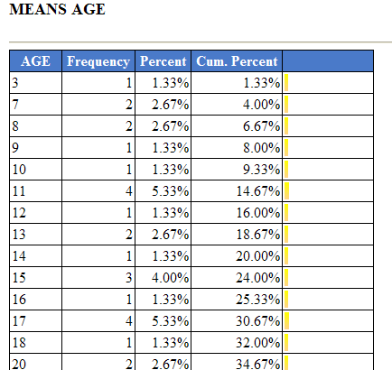
Figure 9.36: Means Output Window
- To view the Descriptive Statistics, scroll down the Age listing.
- Notice the mean age of individuals in the dataset is 36.8.
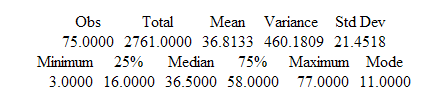
Figure 9.37: Output Data
Try It
For this example, use a numeric variable and a Yes/No variable to determine the MEANS for a group.
- Read in the Sample.PRJ project.
- Click MEANS. The MEANS dialog box opens.
- From the Means of drop-down list, select Age.
- From the Cross-Tabulate by Value of drop-down list, select ILL.
- Click OK. Results appear in the Output window.
- To view the Descriptive Statistics, scroll down the Age listing.
- Notice the Mean Age of those answering yes to ill is 39.2. Those answering no to ill is 32.9.
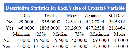
Figure 9.38: Descriptive Statistics Output Window
Other available statistics include:
- ANOVA, a Parametric Test for Inequality of Population Means.
- Bartlett’s Test for Inequality of Population Variances.
- Mann-Whitney/Wilcoxon Two-Sample Test (Kruskal-Wallis test for two groups).
Try It
For this example, use the Classic Analysis Program Editor to create the code.
- Read in the Sample.PRJ project. Open Oswego.
- In the Program Editor window, place the cursor under the Read command created.
Type MEANS Age.- Do not press the Enter key. Leave the cursor on the line of code just created.
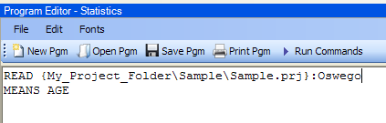
Figure 9.39: Means Age in Program Editor
- Click Run Commands from the Program Editor navigation menu. The code turns gray to indicate execution of syntax.
- Results of the command appear in the Output window.
- Results are the same as those created using the Command Tree dialog boxes.
Use the SUMMARIZE Command
The SUMMARIZE command aggregates data producing an output table showing the descriptive statistics.
SYNTAX
SUMMARIZE varname::aggregate(variable) [varname::aggregate(variable) ...] TO tablename STRATAVAR=variable list {WEIGHTVAR=variable}
- From the Classic Analysis Command Tree, use the READ command to open a PRJ project file.
- From the Classic Analysis Command Tree, click Statistics > Summarize. The Summarize dialog box opens.
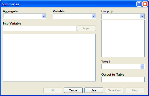
Figure 9.40: Summarize Dialog Box
- From the Aggregate drop-down list, select from the available functions to specify how records will be combined. The options are:
- Average – used only on numeric fields.
- Count.
- First – based on sorts order.
- Last – based on sorts order.
- Maximum.
- Minimum.
- StdDev – Standard Deviation.
- StdDev(Pop).
- Sum – only used on numeric fields.
- Var– Variance – only used on numeric fields.
- Var(Pop).
- From the Variable drop-down list, select from the variables in the dataset.
- In the Into Variable field, type a name to title the summarized variable.
- Click Apply. The code appears in the open field.
- If grouping is necessary, use the Group By drop-down list to select a variable to group the aggregated data.
- If a weight variable exists, use the Weight drop-down list to select a variable to weight the aggregated data.
- In the Output to Table field, type a name for the new data table.
- Click OK. The following message appears in the Output window: Output table created: location listed.
- Click Read/Import. The READ dialog box opens.
- Click the All radio button. All the tables in the dataset appear in a list.
- Locate and select the summary table just created.
- Click OK. The Output window populates with the Record Count for the summary table.
- Use the LIST command to view the summary table.
Try It
- Read in the Sample.PRJ project. Open ADDFull. Three hundred and fifty nine (359) records should be listed in the Output window.
- Click Statistics > Summarize. The SUMMARIZE dialog box opens.
- From the Aggregate drop-down list, select Average.
- From the Variable drop-down list, select the variable GPA.
- In the Into Variable field, type AverageGPA.
- Click Apply. The code appears in the open field.
- From the Group By drop-down list, select the variable GENDER.
- In the Output to Table field, type DATATABLE1.
- Click OK. The following message appears in the Output window:
SUMMARIZE AverageGPA :: Avg(GPA) TO DATATABLE1 STRATAVAR = GENDER
- Click Read/Import. The READ dialog box opens.
- Click the Tables checkbox. All the tables in your dataset appear in a list.
- Select the summary table DATATABLE1.
- Click OK. The Output window populates with a record count of two for the summary table.
- Use the LIST command to view the summary table.
Use the GRAPH Command
The following steps create a basic graph containing one main variable. The GRAPH command opens the Epi Graph application and creates a variety of graph types based on the types of data available in the project.
SYNTAX
GRAPH [<Variable(s)>] GRAPHTYPE ="<GraphType>" [<OptionName>=OptionValue]
GRAPH [<Variable(s)>] * <Crosstab> GRAPHTYPE ="<GraphType>" [<OptionName>=OptionValue]
GRAPH [<Variable(s)>] GRAPHTYPE="<GraphType>" XTITLE="<string>" YTITLE="<string>"
- From the Classic Analysis Command Tree, use the READ command to open an Epi Info 7 .PRJ file.
- From the Classic Analysis Command Tree, click Statistics > Graph. The GRAPH dialog box opens.
- The default graph selection is Bar.
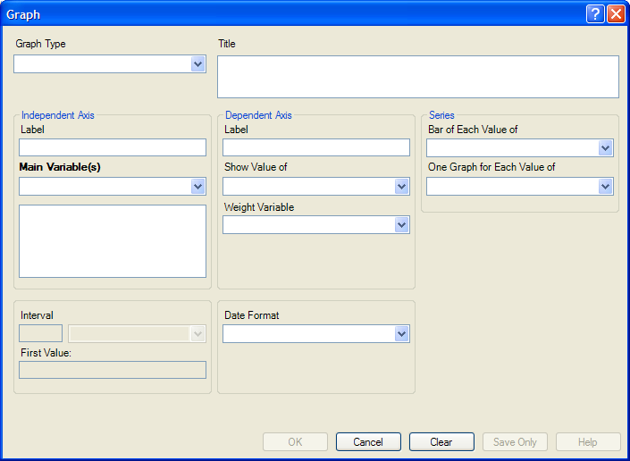
Figure 9.41: Graph Dialog Box
- From the Graph Type drop-down list, select a type of graph from the list.
- From the Main Variable(s) drop-down list, select the X-Axis value to graph. Use the:.
- Show Value Of drop-down list to select an aggregate when multiple records need to be displayed as a group.
- Weight Variable drop-down list to select a variable for weighted Classic Analysis.
- Bar for Each Value Of drop-down list to select a variable to generate multiple series from a single data source, each with a different color or style.
- One Graph for Each Value of drop-down list to select a variable to generate a multiple series from a single data source, each displayed on a separate set of axes.
- X-Axis Label box to type a label to appear in the graph.
- Click OK. Epi Graph opens.
- View the graph. Graphs can be saved by clicking on the floppy disk icon located on the top right hand side of the graph.
- The graph is now embedded in the Output window as part of your output file.
Try It
Create a bar graph using data from the Sample.MDB project.
- Read in the Sample.PRJ project. Open Oswego. Seventy five (75) records should be listed in the Output window.
- Click Statistics > Graph. The GRAPH dialog box opens.
- From the Graph Type drop-down list, select Column.
- From the Main Variable drop-down list, select the variable Age to use for the X-Axis.
- Click OK. Epi Graph opens.
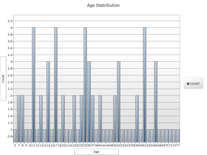
Figure 9.42: Bar Graph
- The bar graph is now embedded in the Output window and part of the output file.
- Notice the Graph code that appears in the Program Editor.