Visual Dashboard: Performing Statistical Analyses with Visual Tools
Visual Dashboard
Analysis Gadgets
Advanced Statistics
Linear Regression
Linear regression is an analysis tool that identifies a relationship between a continuous variable and one or more independent variables. It can be used for simple linear regression (only one independent variable), for multiple linear regression (more than one independent variable), and for quantifying the relationship between two continuous variables (correlation). You can use linear regression when you want to determine the relationship between one dependent variable with one or more independent variables.
In the example below, linear regression is used to determine if systolic blood pressure can be predicted based on an infant’s birth weight and age. The dependent variable is systolic blood pressure, and the independent variables are birth weight in ounces and age in days.
- Set the Data Source to the Sample.PRJ project. Open the BabyBloodPressure form from the Data Source Explorer menu.
- Click OK.
- Right click on the canvas and select Add Analysis Gadget > Advanced Statistics > Linear Regression. The Regression Properties gadget configuration window opens to the Variables property panel. (See the subsequent Linear Regression Properties section for a screen shot of the gadget.)
- From the Outcome Variable drop-down list, select SystolicBlood.
- From the Independent variables drop-down list, select AgeInDays and Birthweight.
- Click OK. The linear regression results appear in the Visual Dashboard canvas.
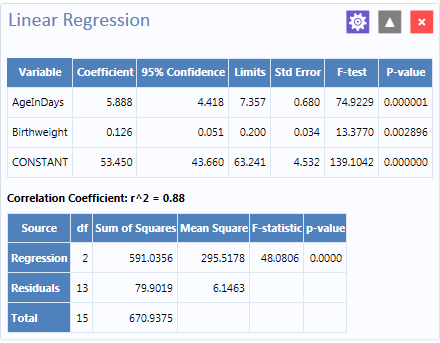
Figure 8.52: Linear Regression results
Coefficients for both independent variables are positive, and the F-statistic associated with each independent variable is highly significant (p-value less than 0.01). These results suggest that each variable (AgeInDays and Birthweight) is a predictor of higher systolic blood pressure.
Linear Regression Properties
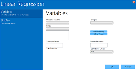
Figure 8.53: Linear Regression gadget
- The Outcome variable is the dependent variable for the regression. The outcome variable must be numeric or a Yes/No field.
- A Weight variable may be selected to use in weighted analyses.
- The Confidence Limits option specifies the probability level at which Epi Info computes confidence limits.
- If the user checks the No Intercept box, the regression is performed without a constant term, which forces the regression line through the origin.
- The Fields drop-down list contains the predictor (independent) variables.
- When selected, the predictor variables will appear in the list box below the Fields drop-down. Double click on a variable to remove it from the list box.
- Click on a variable from the Fields list box to activate the Make Dummy button. If you click Make Dummy, the selected variable will appear in the Dummy Variable list box. Double click on a variable to remove it from the list box.
- Interaction Terms are defined with the Make Interaction button. The Make Dummy button turns to Make Interaction when two or more variables are selected at the same time from the Fields list box (hold the CTRL key to select more than one variable in this list). If you click Make Interaction, the relationship populates the Interaction terms list box. Make Interaction adds all possible combinations of the selected variables to the regression as interaction terms.
Logistic Regression
In Epi Info™ 7, either the M x N/ 2 x 2 table or Logistic Regression may be used when the outcome variable is dichotomous (for example, Ill–Yes/ Ill–No). However, an M x N/ 2 x 2 analysis is useful only when there is one “risk factor,” or explanatory variable. Logistic Regression is useful when the number of explanatory variables (“risk factors”) is more than one. Logistic Regression shows the relationship between an outcome variable with two values and explanatory variables that can be categorical or continuous. To use Logistic Regression, the dependent (outcome) variable must be dichotomous (can be divided into only two parts) Yes/No or numeric 0/1. The independent (other variables) can be numeric, categorical, or Yes/No variables.
Records with missing values are excluded from Logistic Regression analyses. If the Include Missing option is used with missing values and Yes/No fields, dummy variables will generate automatically, contributing Yes vs. Missing and No vs. Missing. Independent variables of text type are automatically turned into dummy variables, which compare each value relative to the lowest value in the sort order. Date or numeric type independent variables are treated as continuous variables unless they are set as dummy variables, which compare each value relative to the lowest value.
The following example uses logistic regression to determine the odds ratio of six foods that could be the cause of a hypothetical foodborne illness. The dependent variable is Ill, and the independent variables are brownbread, cabbage, water, milk, chocolate, and vanilla.
- Set the Data Source to the Sample.PRJ project. Open the Oswego form from the Data Source Explorer menu.
- Click OK.
- Right click on the canvas and select Add Analysis Gadget > Advanced Statistics > Logistic Regression. The Logistic Regression gadget configuration window opens to the Variables property panel. (See the subsequent Logistic Regression Properties section for a screen shot of the gadget.).
- From the Outcome drop-down list, select ILL.
- From the Independent variables drop-down list, select BROWNBREAD, CABBAGESAL, WATER, MILK, CHOCOLATE, and VANILLA.
- Click OK. Results appear on the Visual Dashboard canvas.
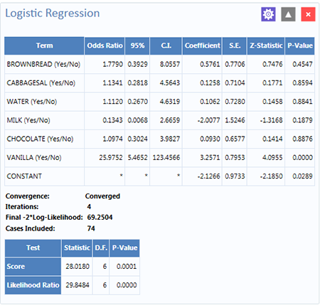
Figure 8.54: Logistic Regression results
The results show that vanilla has an Odds Ratio and Confidence Interval significantly greater than one. This indicates that consumption of vanilla was likely the cause of foodborne illness.
Logistic Regression Properties
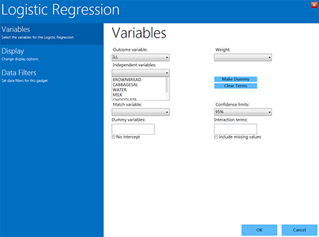
Figure 8.55: Logistic Regression gadget
- The Outcome variable is the dependent variable for the regression. The outcome variable must be numeric or a Yes/No field.
- A Weight variable may be selected to use in weighted analyses.
- Match variable identifies the variable indicating the group membership of each record.
- The Confidence limits option specifies the probability level at which Epi Info computes confidence limits.
- If the user checks the No intercept box, the regression is performed without a constant term.
- The Include missing values setting controls independent variables. If Include missing values is used with missing values and true/false, dummy variables will be created automatically. This will contribute Yes vs. Missing and No vs. Missing. Independent variables of text type are automatically turned into dummy variables that compare each value relative to the lowest value in the sort order. Date or numeric type Independent variables are treated as continuous variables unless designated as dummy values using the Make dummy button. If that occurs, they automatically turn into dummy variables, which compare each value relative to the lowest value.
- The Independent variables drop-down list contains the predictor (independent) variables.
- When selected, the predictor variables will appear in the list box below the Independent variables drop-down. Double click on a variable to remove it from the Other variables list box. Select a variable from the Independent variables list box to activate the Make Dummy button. If you click Make dummy, the selected variable will then appear in the Dummy variables list box. Double click on a variable to remove it from the Dummy variables list box.
- Interaction terms are defined with the Make interaction button. The Make dummy button turns to Make interaction when two or more variables are selected at the same time from the Fields list box (hold the CTRL key to select more than one variable in this list). If you click Make interaction, the relationship populates the Interaction terms list box. Make interaction adds all possible combinations of the selected variables to the regression as interaction terms. Double click on a variable to remove it from the Interaction terms list box.
- The Clear terms button clears all variables from the Dummy variables and Interaction terms list boxes.
Complex Sample Frequencies, Tables, and Means
The Frequency, Table, and Means options in Epi Info™ 7 perform statistical calculations assuming the data were collected using simple random sampling or unbiased systematic sampling. Many surveys also make use of more complex sampling strategies such as stratification, cluster sampling, and the use of unequal sampling fractions. Visual Dashboard provides three options to analyze complex sample data: Complex Sample Frequencies, Complex Sample Means, and Complex Sample Tables.
Generally, in complex sample analysis, there is a variable for the primary sampling unit (PSU) or Cluster from which a sample subject was selected. If the PSUs were chosen from different Strata (e.g., states or counties), there may be a stratification variable (Stratify by). The concept of sample stratification in complex sample design differs from the concept of stratification during epidemiologic analysis using the TABLES command, as the Strata are chosen in the sampling process before analysis. In addition, a weight variable (Weight) is used when sampling strategies result in unequal selection probabilities. The complex sample commands in Epi Info™ 7 can compute proportions or means with standard errors and confidence limits. If a 2×2 table is requested, the odds ratio, risk ratio, and risk difference are provided.
Complex Sample Frequencies
The Complex samples frequencies option produces frequency tables for selected variables. The Sample project contains an Expanded Program for Immunization (EPI) cluster survey. Using the EPI method, a team selected 30 communities (i.e., clusters) from the chosen geographic area and visited each of the 30 communities. In each, they selected seven children in an appropriate age range and determined each child’s immunization (VAC) status. The following example will determine the frequency of vaccinations using Complex Sample Frequencies.
- Set the Data Source to the Sample.prj project.
- Select the Epi1 form from the Data Source Explorer menu.
- Right click on the canvas and select Add Analysis gadget > Advanced statistics > Complex sample frequencies.
- The Complex Sample Frequencies configuration window opens to the Variables property panel.
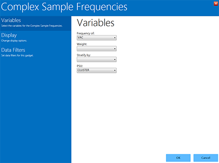
Figure 8.56: Complex Sample Frequencies gadget
Complex Sample Frequencies options are:
- Frequency of identifies the variable(s) whose frequency is computed.
- A Weight variable is selected for use in weighted analyses.
- Stratify by identifies the variable to be used to stratify or group the frequency data.
- The PSU identifies the Primary Sampling Unit.
- From the Frequency Of drop-down list, select VAC (the number of vaccinations received). This will calculate the frequency of vaccinations in the data set.
- From the PSU drop-down list, select CLUSTER (the population group for each case).
- Click OK.
- The Complex Sample Frequencies appear on the canvas.
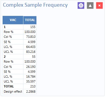
Figure 8.57: Complex Sample Frequencies results
Information provided in the output includes:
- Row % – the row percentage; frequency will always be 100% because the total number of cases will always be 100%.
- Col % – the column percentage. This number represents the frequency computation; in this case, children with 1 vaccination represent 73.810 % and children with 2 vaccinations represent 26.190% out of the 210 total cases.
- SE % – the standard error, which takes into account the complex sample design.
- LCL % – Lower Confidence Limit.
- UCL % – Upper Confidence Limit.
- Total – total number of individuals/elements surveyed.
The results indicate that 73.8% of the 210 children surveyed are vaccinated, with a 95% confidence interval range from 64.4% to 83.2%.
The following example is similar to the one above, except that this is a stratified cluster survey with a separate 30-cluster survey completed in each of 10 strata. To analyze this dataset correctly, we will take into account where each child lives (LOCATION). We will also use a weight variable to account for the differences in population sizes between the different locations.
- Set the Data Source to the Sample.prj project.
- Select the Epi10 form from the Data Source Explorer menu.
- Right click on the canvas and select Add Analysis gadget > Advanced statistics > Complex sample frequencies.
- The Complex Sample Frequencies configuration window opens to the Variables property panel.
- From the Frequency Of drop-down list, select VAC.
- From the Weight drop-down list, select POPW (the percent of the total population in each cluster).
- From the Stratify By drop-down list, select LOCATION.
- From the PSU drop-down list, select CLUSTER.
- Click OK.
- The Complex Sample Frequencies results appear on the canvas.
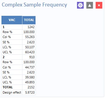
Figure 8.58: Complex Sample Frequencies stratified and weighted results
The results indicate that 55.3% of the 2,152 children surveyed are vaccinated, with a 95% confidence interval range from 50.1% to 60.4%.
Complex Sample Means
The Complex Sample Means command can be used when the outcome variable is continuous, such as age, cholesterol level, etc. You can either calculate an overall mean with its measures of variation or compare means across a grouping variable. As an example of calculating means with a grouping variable, use the data from the Smoke form located in the Sample project folder. In this example, the investigator is interested in determining if, among smokers, there is a difference in the average number of cigarettes smoked between males and females. In these data, the variable SEX is coded as 1=male and 2=female.
- Set the Data Source to the Sample.prj project.
- Select the Smoke form from the Data Source Explorer menu.
- Right click on the canvas and select Add Analysis gadget > Advanced statistics > Complex sample means.
- The Complex Sample Means configuration window opens to the Variables property panel.
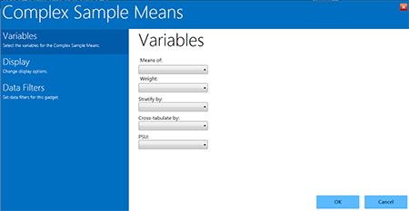
Figure 8.59: Complex Sample Means gadget
Complex Sample Means options:
- Means of identifies the variable for which the mean is being computed.
- A Weight variable is selected for use in weighted analyses.
- Stratify by identifies the variable to be used to stratify or group the frequency data.
- Cross-tabulate by identifies the variable to be used to cross-tabulate the main variable.
- The PSU identifies the Primary Sampling Unit.
- From the Means Of drop-down list, select NUMCIGAR (number of Cigarettes smoked).
- From the Weight drop-down list, select SAMPW (calculated based on sample size and population size).
- From the Stratify By drop-down list, select Strata.
- From the Cross-tabulate By drop-down list, select Sex.
- From the PSU drop-down list, select PSUID.
- Click OK.
- The Complex Sample Means results appear on the canvas.
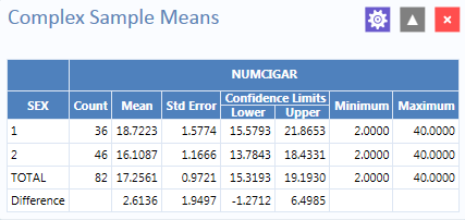
Figure 8.60: Complex Sample Means results
The results indicate that among the 82 individuals who smoked cigarettes, the average number of cigarettes smoked per day (NUMCIGAR) for men was 18.7, and 16.1 for women, with a 95% confidence interval range of 15.6 to 21.8 for men and 13.7 to 18.4 for women. Note that the Smoke file has 337 individuals (this value is shown in the upper right hand corner of the canvas). However, the number of cigarettes smoked per day has data for only the 82 smokers. For nonsmokers, this variable was left blank and is therefore treated as missing data and excluded from analysis.
Complex Sample Tables
The Complex Sample Tables option in Visual Dashboard allows you to specify an Exposure Variable and an Outcome Variable. The following example uses Complex sample tables to show whether the mother receiving prenatal care (PRENATAL) has an effect on the child’s vaccination status. If the mother had received prenatal care, PRENATAL=1, else PRENATAL=2.
- Set the Data Source to the Sample.prj project.
- Select the Epi10 form from the Data Source Explorer menu.
- Right click on the canvas and select Add Analysis gadget > Advanced statistics > Complex sample tables.
- The Complex Sample Tables configuration window opens to the Variables property panel.

Figure 8.61: Complex Sample Tables gadget
Complex Sample Tables options:
- Exposure identifies the variable that will appear on the horizontal axis of the table. It is considered to be the risk factor.
- Outcome Variable identifies the variable that will appear on the vertical axis of the table.
- A Weight variable is selected for use in weighted analyses.
- Stratify by identifies the variable to be used to stratify or group the frequency data.
- The PSU identifies the Primary Sampling Unit.
- From the Exposure drop-down list, select PRENATAL.
- From the Outcome drop-down list, select VAC.
- From the Weight drop-down list, select POPW (the percent of the total population in each cluster).
- From the Stratify By drop-down list, select Location.
- From the PSU drop-down list, select Cluster.
- Click OK.
- The Complex Sample Tables results appear on the canvas. You may need to scroll down to see the full results.
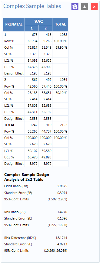
Figure 8.62: Complex Sample Tables results
The results show that 60.7% of children whose mothers received prenatal care were vaccinated, compared to 42.6% of those children whose mothers did not receive prenatal care.
The 2 x 2 data shows that the odds ratio in the data was 2.088, the risk ratio was 1.427 and this risk difference is 18.2%. The prevalence (risk) ratio indicates that 1.427 times as many children of women who received prenatal care were vaccinated (60.734% divided by 42.560% = 1.427), compared to children born to women who had not received prenatal care—a 40% difference.