At a glance
At CDC's Center for Forecasting and Outbreak Analytics, we are building modeling tools and computational pipelines so that we can do complicated data analyses quickly and accurately in response to epidemics. Our goal is to make these tools accessible to federal, state, tribal, territorial, local, and academic partners. One of these efforts is to estimate the time-varying reproductive number, Rt, a measure that helps us quickly assess whether infections are increasing or decreasing.
As of May 2024
Data Update
COVID-19 Growth Estimates
Current Epidemic Growth Status based on Rt for States and Territories
Measuring Transmission with Rt
The basic reproductive number, R0 (pronounced R-naught), is defined as the expected number of new infections caused by each infected person in a fully susceptible population and in the absence of interventions. R0 is an important theoretical concept in epidemiology, but in the real world, a fully susceptible population rarely exists. The time-varying effective reproductive number is known as Rt. When Rt is above one, infections are increasing, and when Rt is below one, infections are decreasing.
What Rt can and cannot tell us:
What Rt cannot tell us: Rt cannot tell us about the underlying burden of disease, just the trend of transmission. An Rt< 1 does not mean that transmission is low, just that infections are decreasing. It is useful to look at respiratory disease activity in conjunction with R
What is the Time-Varying Effective Reproductive Number, Rt
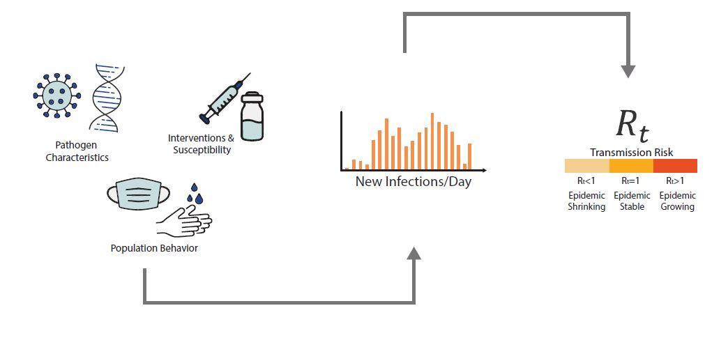
An epidemic's growth and decline are driven by underlying changes in transmission over time. Early in an epidemic of a novel disease, when everyone is susceptible, transmission rates are usually highest, and then decline as people change their behavior to avoid infection or gain immunity through infection or immunization. The peak of an epidemic is a turning point that occurs when transmission falls below a critical threshold where, on average, each infected person no longer causes more than one new infection. Rt is defined as the average number of new infections caused by each infected person at time t, usually measured in days. Rt tells us whether at that time, infections are increasing, decreasing, or staying relatively flat. We estimate Rt from data, and it accounts for current levels of population susceptibility, interventions, and behavior at the time the underlying infections occurred (Fig. 1). During an epidemic, Rt estimates provide information about the growth status of the epidemic and can be used to forecast short-term changes in cases, hospitalizations, or deaths, and to assess the effectiveness of interventions designed to slow transmission.
For Public Health Professionals and Epidemiologists - Learn More About How We Estimate Rt
See Video featuring CDC Scientist Katie Gostic on how to calculate Rt
Let's imagine a world in which we can observe every disease transmission event exactly when it occurs. In this hypothetical world, we count the number of new infections that occurred on day t and divide by the number of infected persons who caused them, to give us Rt: the average number of new infections that each previously infected person caused (Fig. 2).

In reality, it's almost impossible to know exactly when transmission occurred or who infected whom in epidemiological data. While sometimes epidemiologists run focused studies designed to observe transmission events and transmission chains, these studies require intensive monitoring of a small group of participants and are the exception, not the rule. To get around these challenges, we estimate Rt using data that are relatively easy to obtain: daily counts of the number of new cases, hospitalizations, or deaths. We input these data into a mathematical model designed to deal with three main challenges of data observation:
- We almost never know who infected whom
- There is a lag between the moment someone is infected (an unobservable event) and the date their infection could become observable and/or reported, e.g., as a symptomatic case, a positive test, or hospitalization
- Not all infections will be observed. For example, not all cases will have symptoms and not all cases who have symptoms will be tested or hospitalized
Below, we'll walk through the basic logic, assumptions, and weaknesses of this model. The technical details of our approach are described (here).
To estimate Rt we need to divide the total number of newly infected people on day t by the number of people who caused those infections (Fig. 2). But how can we do this if the data only contain counts of the total numbers of infections observed each day?
Note
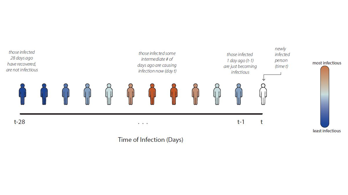
In count data, we can directly read the numerator of the Rt ratio, the number of newly infected people on day t, from the data. The denominator is more difficult to assess. Instead of trying to infer exactly who infected whom, we make assumptions grounded in infectious disease biology. For COVID-19, for example, we know that individuals infected yesterday are just becoming infectious as their viral loads increase. Meanwhile, individuals infected weeks ago have likely recovered and are no longer infectious.* We can assume that individuals who were infected some intermediate number of days in the past are now causing the bulk of new infections (Fig. 3).
To estimate Rt, we must develop a model that turns the assumption "individuals infected some days in the past are the ones causing transmission now" into an equation. Our equation is a more complex version of the Rt ratio in Fig. 1, inferred using observable variables. To count the number of individuals in the infector generation on day t, we need to sum across all the individuals who became infected in the recent past – starting yesterday and going back weeks ago – weighted by their current infectiousness. For COVID-19, we assume that individuals infected between 1 and 7 days ago are most infectious,* but individuals infected earlier or later may still cause infections. For details of our Rt equation, see Fig 4.
*Day 1-7 covers the central 95% of the generation interval distribution for Omicron from Park et al., 2023; and day 1-5 covers the central 80% of the generation interval distribution. See Figure 5 for a definition of the generation interval.

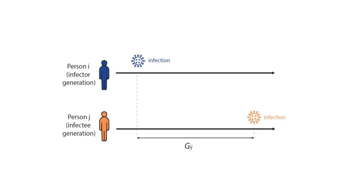
To formally estimate how long the expected wait between infections in a chain of transmission is – and to establish the infectiousness weighting function in Fig. 4 above – infectious disease models use a distribution called the generation interval (G), defined as the interval between the infection times of an infector-infectee pair (Fig 5). For example, if person i was infected on Monday, and if person i infects person j on Friday, then the Gij is four days. We know that the generation interval varies between transmission pairs, and so we want the distribution of times between infector-infectee pairs. We can estimate the generation interval distribution using data from household or contact tracing studies, in which the approximate timing of infections is observed, or by using the serial interval (the time between onset of symptoms of an infector-infectee pair) as a proxy.
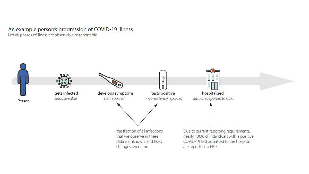
When we estimate Rt, we want to know how many new infections occur on day t. In the real world, we observe events that occur days to weeks afterwards like cases, hospitalizations, or deaths (Fig. 6). These delays are unavoidable and fall into two main categories:
- Biological delays between the moment a person is first infected and the moment their infection could become observable and/or reportable as a confirmed case, hospitalization, or death.
- Reporting delays. Let's focus on hospitalization as the observable event because at CDC we currently estimate Rt for COVID-19 and influenza using counts of daily hospital admissions. Individuals transit through many stages of illness from infection to symptomatic illness to testing positive (by either a home test or a PCR test in a health care setting), and some then become hospitalized (Fig. 6). Currently, hospitalization data are one of the most complete and reliable data sources for COVID-19 and influenza. We do not currently have timely, reliable or complete counts of individuals with symptomatic illnesses or positive tests.
Caveats and complications:
- On the most recent dates, we have not yet observed all infections that have occurred, as some infected people have not yet developed symptoms or been hospitalized. This is a challenge because people are usually most interested in recent trends, but recent data are incomplete.
- There are day-of-week effects in healthcare visits and reporting, where the data consistently show more reports on weekdays vs. weekends.
- Hospitalizations are not always reported on the day that they occur. For example, sometimes test results take a few days to come back from the lab, diagnoses undergo review, or there are delays in transferring data.
To adjust for incomplete reporting on recent dates, CDC is implementing "nowcasting" approaches. Essentially, we can look back at past reporting patterns to estimate the fraction of total reports that were observed 1, 2,..., n days after the reported event. Then we can scale up accordingly to estimate the number of events that will eventually be reported on each day.
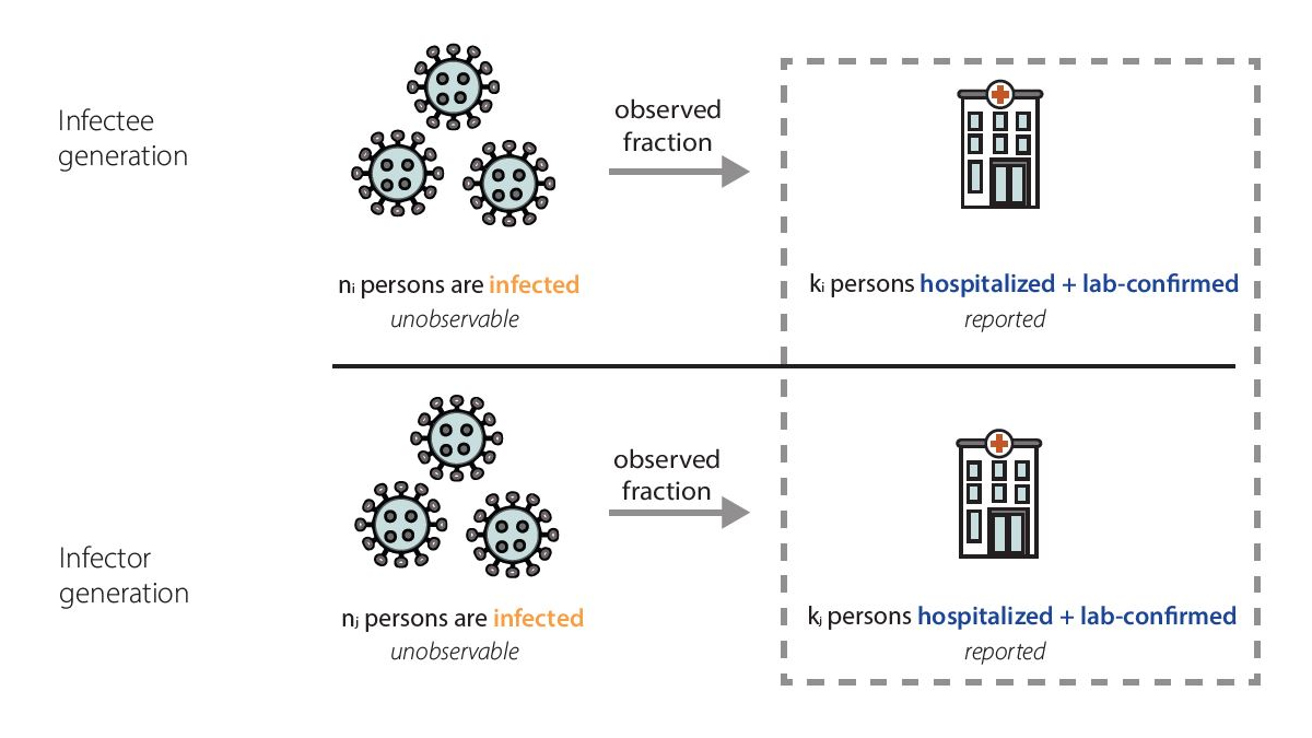
In our data, we only observe the fraction of infected individuals that were admitted to the hospital and tested positive (Fig. 7). Because facilities are currently required to report individuals with laboratory-confirmed COVID-19 and influenza who are admitted to the hospital, we think that the fraction of infections we observe as laboratory-confirmed hospitalizations is quite stable.

Mathematically, we expect our Rt estimates to be unbiased as long as the fraction of observed infections in hospitalization data is not changing rapidly. That is because the observed fraction impacts both the numerator – the infectee generation – and denominator – the infector generation – of our Rt equation equivalently (Fig. 8). In reality, there is probably no epidemic dataset where there is no change at all in the fraction of observed infections over time. We have chosen to focus on hospitalizations because we think that using hospitalizations, we observe one of the most stable fractions of infections of any available data source (Sherratt et al., Richardson et al.) (Fig 6). There are some situations where the fraction of observed infections could change quickly enough to temporarily cause biases in Rt estimates, such as the emergence of a more severe variant, lack of diagnostic tests, or a clinical or testing practice change within a healthcare setting. If such a situation occurs, we will flag the estimates we publish noting that there is some possibility of inaccuracy during the brief period before the fraction observed re-stabilizes.
It is important to note that hospitalized individuals are systematically different from the general population; for example, they tend to be older for COVID-19 and influenza-related hospitalizations. Furthermore, severe infection and hospitalization fundamentally change a person's behavior in ways that probably affect their opportunities for onward transmission. However, these differences in age, behavior, and contacts don't directly affect our estimates, because we are not measuring the number of new infections that hospitalized individuals go on to cause. Instead, our estimates reflect the population average level of transmission that caused those individuals to become hospitalized themselves.
In fact, though counterintuitive, mathematically, in an epidemic system without rapid changes in severity, infectiousness, or precautionary behavior, different age groups should experience roughly similar epidemic growth rates over time after an initial mixing period. While early in the COVID-19 pandemic these conditions were probably not met, at this point, we believe these effects are minor. Although the total number of infections in each group will be different, the relative change should be the same. This means that estimates of Rt based on incident events from a subgroup (individuals who are hospitalized, for example) of a population are unbiased as long as the fraction of observed infections in hospitalization data stays roughly constant.
| COVID-19 | Influenza | |||
| Rt Estimation Model | EpiNow2
We use the package default priors defined on the package website except where otherwise noted:
Rt=0: Mean: 1, standard deviation (sd): 0.2 (This is the initial Rt)
αsd: 0.0075 (This is the prior on the standard deviation of the gaussian process) |
EpiNow2 Documentation;
|
same specification as for COVID-19
|
|
| Generation interval distribution | Lognormal distribution with [unit scale] Mean: 2.9 days, sd: 1.64 days (95% CI 0.92 – 7.1), with maximum 12 days and a minimum of 1 day | Park et al. 2023*
(Omicron-specific)
|
Gamma-distribution with mean: 3.6 days, sd: 1.7 days, with maximum 9 days and a minimum of 1 day | Cowling et al. 2009 |
| Incubation period distribution
|
Modified Weibull distribution with mean 4.24 days, 95% CI (3.6-4.9) | Park et al. 2023*
(Omicron-specific)
|
||
| Symptom onset to hospitalization distribution | Fitted negative binomial distribution with mean: 6.99 days, overdispersion parameter: 2.49 | Danaché et al, 2022 | Gamma-distribution with mean: 3.52 days, sd: 2.91 days | Internal data |
| Delay Distribution | Combined incubation and hospitalization onset distribution: mean: 12.18 days sd: 5.67 days | Derived from incubation period and symptom onset to hospitalization | ||
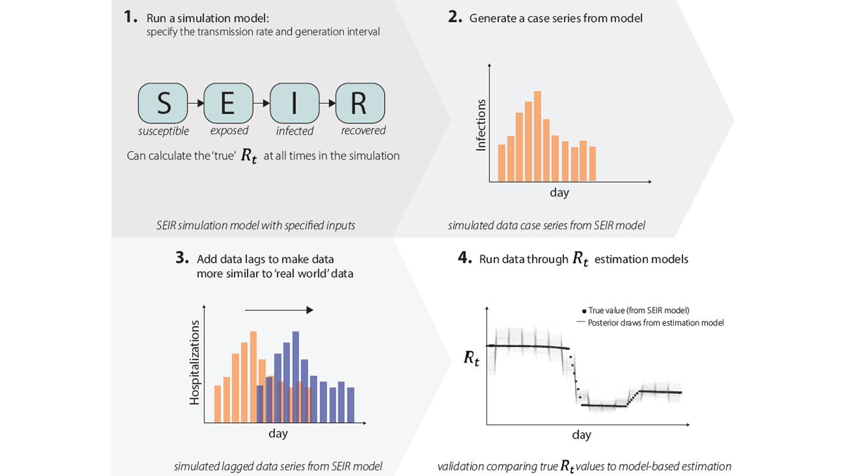
In some epidemic modeling analyses, we get to check our answers. For example, if we generate a short-term epidemic forecast, we can wait a few weeks, and then check our predictions against what really happened. But we're never able to observe Rt directly, and so we don't have a gold standard source of truth to check our models against. As a result, we use a few different methods to check that our estimates are reliable.
- We run simulation studies. We run an epidemic simulation using a dynamic mathematical model with four compartments: susceptible (S), exposed (E), infected (I), and recovered (R) (Fig. 9.1) where we can calculate the 'true' Rt value at all times. The simulation produces an epidemic time series with counts of the number of new infections per day (Fig. 9.2), and we add lags to these data to make them more similar to the case, hospitalization, or death data that we observe in the real world (Fig. 9.3). We can run these simulated data through our Rt estimation models just like real data, only in this case we know exactly what the answer (Rt) should be, as we specified it when simulating the data. We then compare results to the correct answers (Fig. 9.4). If our models do not accurately estimate Rt, we know we need to make changes, until the model accurately estimates Rt.
- We run a few different Rt estimation models side by side, and we check their answers against each other. We don't expect different models to give the same answer, but we do expect the answers to be similar. If they're not, we investigate, and make changes if needed.
- We perform common sense checks. If the data show that the epidemic is growing rapidly, then we should see Rt estimates, including confidence intervals, above one for the corresponding time period, after adjusting for lags.
- We evaluate short-term forecasts from our models. The R software package we use to do Rt modeling, EpiNow2, has produced forecasts that have been submitted to both the CDC and ECDC COVID-19 forecasting hubs, and we are currently further validating these forecasts as part of this season's FluSight Challenge.
Key Takeaways
Key Points
Rt is a transmission metric that estimates the ratio of infected to infectors in an epidemic at a particular point in time. Rt estimates help inform situational awareness, giving clues as to how quickly an epidemic is likely to increase or decrease in the near future. Rt estimates can even form the backbone of quantitative short-term epidemic forecasts. To be useful for decision making, Rt estimates need to be accurate, accounting for time lags because transmission events causing cases now occurred days to weeks ago.
Especially in a novel outbreak, it is essential to know whether the epidemic has started, if we are nearing a peak, and/or if transmission has begun to decline. Rt allows policy-makers and public health decision-makers to assess the impact of interventions, because it estimates how transmission rates have changed over time, and to assess the intensity of spread, because it directly reflects growth in infections.

What’s next?
We are starting with Rt estimation for respiratory viruses in collaboration with the National Center for Immunization and Respiratory Diseases, but in the long term, we plan to build a well-tested analytic infrastructure that we could use to estimate Rt for a novel pathogen in a future infectious disease epidemic. Even for something like Rt, where the quantity we're trying to estimate is conceptually relatively simple, it takes incredible care and complicated modeling tools to adjust data as they are observed and obtain accurate estimates quickly. We are also exploring new models that will allow us to combine wastewater data with other signals when we estimate Rt. It is incredibly difficult to build these kinds of analytic pipelines on the fly. Investing the time now to build good infrastructure and think through the problems we can anticipate will leave us better prepared for the next infectious disease epidemic.
- Day 1-7 covers the central 95% of the generation interval distribution for Omicron from Park et al., 2023; and day 1-5 covers the central 80% of the generation interval distribution. See Figure 5 for a definition of the generation interval.