Advanced Tutorial on Wireless Communication and Electronic Tracking: Appendix B
B.1 Basic Equations
B.1.1 Power Conversions
Power values are expressed either in watts (W) or milliwatts (mW). The power in W may be converted to mW using the following equation:
where
pmW = power (mW),
pW = power (W)
The power in mW may be converted to W by solving the above equation for pW.
Power values are often expressed in decibels with respect to a milliwatt, abbreviated dBm. The power in watts may be converted to dBm using the following:
where
PdBm = power (dBm)
pW = power (watts)
A positive value indicates more than one milliwatt, whereas a negative value indicates less than one milliwatt.
The power in dBm may be converted to watts using the following:
where all terms were identified previously.
B.1.2 Antenna Gain Conversions
Antenna gain is often given in dBi units (The "i" stands for isotropic, a perfect point source which radiates in a spherical manner). To convert dBi to a numeric value, use the following equation:
where
g = numeric antenna gain (dimensionless)
G = antenna gain (dBi)
Given the numeric antenna gain, the gain in dBi may be computed as follows:
where all terms were identified previously.
B.1.3 Wavelength
An electromagnetic (EM) signal has a frequency and a wavelength. Given the frequency, the wavelength may be computed using the following approximate equation:
where
λ = wavelength (meters)
f = frequency (MHz)
B.2 Near-Field/Far-Field Distances
The radiation characteristics of an antenna vary with distance from the antenna. For instance, at large distances (referred to as the far-field region) some radiation characteristics are independent of distance, e.g., the gain is constant as the distance increases. On the other hand, at distances closer to the antenna (near-field region), the gain changes with distance.
When two antennas are in the far-field of each other, the activation of one antenna has no effect on the performance characteristics (e.g., impedance, radiation pattern) of the other antenna. Conversely, when the antennas are in the near-field of each other, the activation of one antenna could modify the performance characteristics of the other antenna.
For low-gain types of antennas (monopole, dipole, whip, rubber ducky), a common minimum value for the distance to the far-field region is four wavelengths. For directive types of antennas (e.g., Yagi-Uda), the distance to the far-field region may be calculated using the following equation:
where
DFF = distance to the far-field region (meters)
Dant = largest dimension of the antenna (meters)
λ = wavelength at the system’s frequency (meters)
B.3 Incident Radiation
An EM wave consists of an electric field (E-field) and a magnetic field (H-field). In general, the E-field and the H-field are perpendicular to each other and to the direction (the ray path) that the wave is traveling. The intensity of either field is referred to as field strength, where the intensity of the E-field is measured in volts per meter (V/m) and the intensity of the H-field is measured in amperes (amps) per meter (A/m). The E-field and the H-field together carry power, where the power flow through space is called the power density, which is measured in watts per square meter (W/m2).
B.3.1 Effective Isotropic Radiated Power
The effective isotropic radiated power (EIRP) is the defined as the amount of power leaving the antenna into the environment. The EIRP is measured at the output of the antenna and is computed as follows:
where
EIRP = effective isotropic radiated power (dBm)
PT = transmitter power (dBm)
LLT = line loss (dB)
GT = transmit antenna gain (dBi)
If peak transmitter power is used in the above, the result will be peak EIRP; if average transmitter power is used in the above, the result will be average EIRP.
B.3.2 Power Density
The power density s, in mW per square meter (mW/m2) incident on a point may be computed using the following equation:
where
s = power density (mW/m2)
pT = transmitter power (mW)
gT = transmit antenna gain (near-field or far-field) (dBm)
R = distance from the antenna to the point of interest (m)
The power density in dBm per square meter (dBm/m2) may be evaluated using the following equation:
where
S = power density (dBm/m2)
and all other terms were defined previously.
The power density equations B-9 and B-10 assume that the EM wave radiated by a transmit antenna spreads as in a spherical wave. This is not strictly true in a tunnel; consequently the resulting values are estimates.
B.3.3 Electric Field Strength
Given a value for the power density incident on a point, the intensity of the electric field may be computed using the following equation:
where
E = root-mean-square (rms) E-field strength (V/m)
s = power density (W/m2)
120π (~377) = impedance of free space (dimensionless)
B.3.4 Magnetic Field Strength
Given a value for the power density incident on a point, the intensity of the magnetic field may be computed using the following equation:
where
H = root-mean-square (rms) H-field strength (A/m)
and all other terms were defined previously.
B.4 Electromagnetic Propagation
B.4.1 Free-Space
In general, when two antennas are within line-of-sight of each other, and in the far-field of each other, the level of received power is related to the free-space propagation loss. This loss assumes the EM wave radiated by a transmit antenna spreads spherically. In the absence of a detailed propagation model, the free-space propagation loss may be used to provide an estimate of the loss. The free-space propagation loss along the straight-line path between two antennas may be calculated using the following equation:
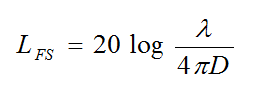
where
LFS = free-space propagation loss (dB)
Free-space propagation losses do not include any additional diffraction and reflection losses (e.g., reflection, multipath, refraction) along the ray path.
λ = wavelength at the receive frequency (m)
D = distance between antennas (m)
B.4.2 Tunnel Modeling
In general, the propagation loss should include all of the possible elements of loss associated with interactions between the propagating wave and any object between transmit and receive antennas inside of the mine. There are propagation models that predict the loss for a long or narrow rectangular mine tunnel. It is important to mention that the EM propagation model for mines should include the dimensions of the mine, the dielectric constants of the walls and roughness of the walls, and the model should be validated with measured data obtained from a mine.
B.4.2.1 Straight Rectangular Tunnel
Suppose a three-dimensional (3-D) straight rectangular tunnel has a width of a and a height of b (both a and b are in meters), as shown in Figure B.4-1.
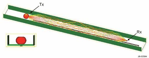
The propagation loss can be modeled [JSC 2008a] as following free-space loss up to a breakpoint distance, and then following a linear decay rate for distances beyond the breakpoint. The propagation loss depends on the polarization of the wave. Only the EM wave polarization that experiences the least amount of attenuation as it propagates through the tunnel is of interest, because this is the wave that will travel the furthest. The polarization that is attenuated the least corresponds with the dimension of the tunnel which is greatest; if the width is greater than the height, then the attenuation of the horizontal polarization is lower than for the vertical polarization. The propagation loss and maximum propagation distance can be calculated as follows:
- Find the breakpoint distance, dFSL, in meters using the following equation:
 (B14)
(B14)where b and λ are in meters.
- Find the free space loss, FSLbp, in dB at the breakpoint distance dFSL using the following equation:
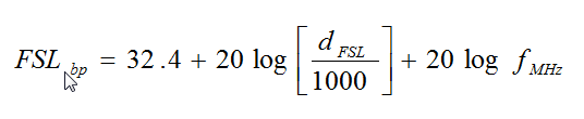 (B15)
(B15)where
dFSL = breakpoint distance, (m)
fMHz = the frequency (MHz). - Determine the far-zone linear decay rate, αspe, in dB/m from the following equation:
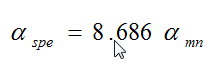 (B16)
(B16)where αmn is given by:
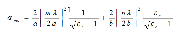 (B17)
(B17)where
εr = relative dielectric constant of the wall (typical value is 6)
λ = wavelength (m)
m,n = the mode numbers of the propagation loss inside of the mine. The least attenuated modes, also known as fundamental modes, are when m=1 and n=1.Note: Equation B-17 is used when b > a. If a > b then the same equation is used but a and b are interchanged in the equation.
- Find the median path loss as a function of the distance d, where d is in meters:
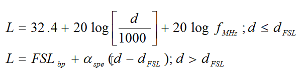 (B18)
(B18) - When the maximum allowable link path loss (Lmax) is known from the radio and reliability parameters, the following relation may be used to find the corresponding maximum link distance dmax (assumed here to be greater than the break point distance dFSL):
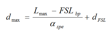 (B19)
(B19)
B.5 Link Budget Analysis
The objective of a link budget analysis is to catalog all the losses and gains between the two ends of a communication link, thus obtaining the maximum loss in signal strength that can be tolerated between a transmitter and receiver. This maximum allowable loss in signal strength is also known as the available path loss. It is specified in logarithmic units (dB) and can in turn be translated into the greatest spatial distance between transmitting and receiving antennas, at which reliable communication of the desired quality can still take place. In the context of wireless mobile communications systems, link budgets are a prerequisite to determining the location of, as well as spacing between, antennas or nodes in order to ensure reliable and uninterrupted communication as miners move through an area of intended radio coverage.
This subsection describes the method for computing a link budget when a transmitter is attempting to communicate with a receiver.
B.5.1 Desired Received Power
B.5.1.1 Far-Field
When two antennas are in the far-field of each other, the level of desired received power may be computed using the following equation:
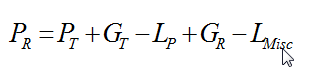
where
PR = received desired signal power (dBm)
PT = transmitter power (dBm)
GT = transmit antenna gain (dBi). GT is the gain in the direction of the propagation ray path.
LP = total propagation loss between antennas (dB). LP is evaluated at the receive frequency, and includes any additional losses (diffraction, reflection, absorption, etc.) along the ray path between antennas.
GR = receive antenna gain (dBi). GR is the gain in the direction of the propagation ray path.
Lmisc = total of any additional miscellaneous losses (dB). Lmisc could include losses either at the transmitter or at the receiver. Examples of such terms are transmission line loss, insertion loss, filtering loss, or any other miscellaneous system loss.
The above equation is the general equation to be used for desired signal link analysis.
B.5.1.2 Near-Field
In general, when two antennas are within line-of-sight of each other, and in the near-field of each other, it is not possible to separate the propagation loss and the antenna gains into individual terms as in the received power equation (Equation B-20). In this case, ignoring any miscellaneous losses, the level of received power may be computed using the following equation:
where
PR = received signal power (dBm)
PT = transmitter power (dBm)
C = coupling evaluated at the receive frequency (dB)
The coupling term, C, must be evaluated using numerical EM software (e.g., Numerical Electromagnetics Code (NEC)) , the details of which are beyond the scope of this tutorial.
B.5.2 Receiver Effective Noise
Many communication receivers are of the superheterodyne type, where the receiver includes several stages, namely, a radio frequency (RF) stage, and one or more intermediate frequency (IF) stages. Analysis is often performed using the level of desired signal at the IF stage having the narrowest bandwidth. This is usually the final IF stage, although this is not always the case.
Electronic circuits, such as in a receiver, generate electrical noise which is referred to as thermal noise. The thermal noise is present at each stage of the receiver. Ignoring any external noise sources, the effective input noise power level at an IF stage is given by:
where
NT = receiver’s effective input thermal noise power, ignoring any external noise (dBm)
k = Boltzmann’s constant (1.38 x 10⁻²³ J/°K)
T = absolute temperature, in degrees Kelvin. The standard value is 290°K (62.3°F).
B = bandwidth of the IF stage (Hz)
fn = receiver’s noise factor (unitless)
The noise factor accounts for additional noise contributions from other stages of the receiver. The receiver noise figure (NF) is 10 times the log of the noise factor. A typical value of 6 dB may be used for the NF.
In an underground mine, electrical noise is generated by sources in the various pieces of mining equipment (e.g., electric motors, belt drives, breaks in power line insulation, etc.). This noise is referred to as man-made noise or environmental noise. Environmental noise in the passband of the receiver enters the receiving antenna, passes unattenuated through the stages of the receiver, and adds to the thermal noise. Including any environmental noise, the effective input noise power level at an IF stage of a receiver may be computed as follows:
where
N = receiver's effective input noise power including any external noise (dBm)
ne = environmental noise power in the mine (W)
and all other terms were defined previously.
Note in Equation B-23 that the total level of noise must be found by adding the individual noise contributions in watts.
B.5.3 Signal-Noise Ratio (SNR)
The SNR is useful in desired-signal analysis and may be found as follows:
where
SNR = available signal-to-noise power ratio (dB)
S = signal power (dBm)
N = receiver effective noise power level including any external noise (dBm)
When S is a measurement or prediction of the available received signal level under certain conditions, then SNR is the available SNR.
B.5.4 Receiver Sensitivity
The method for determining receiver sensitivity depends on whether the receiver is designed for analog signals or for digital signals. As indicated previously, an analog signal is one where the signal is continuous over time, and a digital signal is one where the signal is discontinuous over time.
In order for a receiver to detect a desired signal, the signal needs to be higher than the level of the effective receiver noise. Receiver sensitivity is defined as the power level in dBm required for some particular standard response for the receiver. The sensitivity level for a receiver may be computed using the following:
where
S = receiver sensitivity (dBm)
N = receiver effective noise power level (dBm)
SNRreq = required signal-to-noise power ratio (dB)
Note that the SNR in the above equation is a required SNR, which is different than the available SNR mentioned in the previous subsection.
The next two subsections define methods for determining the required SNRs for analog and digital receivers.
B.5.4.1 Analog Receivers
In an analog receiver, sensitivity is usually defined as the power level in dBm required for a certain level of signal intelligibility.
For voice communications, the articulation score (AS) is defined as the percentage of words, phrases, sentences, or other message elements that have been correctly identified. The AS is usually evaluated by a listener panel [JSC 2006]. The articulation index (AI) is a calculated quantity, ranging from 0.0 to 1.0, and is designed as a predictor of signal intelligibility. For daily working conditions, where the noise levels might be significantly raised due to the mine equipment, the minimum level for AI might be 0.8 or 0.9. In a rescue situation, the minimum AI level might be 0.95, because the mine equipment would likely be off, so the environmental noise levels would be lower.
The sensitivity criterion is the difference between the sensitivity and the effective receiver noise level. For an analog system, the sensitivity criterion is generally a required SNR in dB.
The sensitivity criterion depends on the modulation type of the receiver. The curves of the required SNR for various analog modulation types as a function of the AI are available [JSC 2006]. A value of 0.9 was selected for the minimum acceptable AI level. Approximate required SNR levels in the presence of noise only are listed in Table B.5-1. If the modulation type is unknown, the minimum typical required SNR for an analog system would be 12 dB.
| Modulation Description | Min AI | Required SNR (dB) |
|---|---|---|
| Double sideband AM voice | 0.9 | 29 |
| Single sideband AM voice | 0.9 | 16 |
| FM voice | 0.9 | 13 |
B.5.4.2 Digital Receivers
In a digital receiver, sensitivity is usually defined as the power level in dBm required for a specified maximum fraction of errors in the detected pulses or data bits, i.e., the bit error rate (BER). Depending on the application, a typical required BER might be one error in ten thousand bits, or 10-4.
For digital systems, an important parameter is Eb/No, which is the required energy per bit relative to the noise power. The Curves of the required Eb/No as a function of the required BER for various digital modulation types are available [JSC 2006]. To convert from Eb/No to SNR, use the following equation:
where
SNRreq = required SNR (dB)
Eb = energy required per bit of information (joules or watt-second (W-s))
No = thermal noise density in 1 Hz of bandwidth (W/Hz)
Rb = system bit rate (data rate), in bits/s (or Hz)
BR = receiver IF-stage bandwidth (Hz)
The parameter No may be found by using the following:
where
N = receiver effective noise level (dBm)
BR = receiver IF bandwidth (Hz)
If the IF-stage bandwidth, BR, is not known, it may be estimated from the modulation type and the system bit rate. Table B.5-2 lists typical receiver bandwidths for selected digital modulation types. The receiver bandwidth is given in terms of a multiple of the system bit rate (Rb).
| Modulation Type | Bandwidth BR (Hz) |
|---|---|
| BPSK | 1*Rb |
| QPSK | 0.5*Rb |
| 8-PSK | 0.333*Rb |
| 4-QAM | 0.5*Rb |
| 8-QAM | 0.333*Rb |
| 16-QAM | .25*Rb |
As for analog systems, the sensitivity criterion depends on the modulation type of the receiver. Given a value of the BER, the required Eb/No may be determined from curves for various digital modulation types [JSC 2006]. A value of 10-4 was selected for the maximum acceptable BER level. Approximate required Eb/No levels in the presence of noise only are listed in Table B.5-3.
| Modulation Description | Max BER | Required Eb/No (dB) |
|---|---|---|
| PSK, 1 bit per symbol (BPSK) | 10-4 | 8.5 |
| PSK, 2 bits per symbol (QPSK) | 10-4 | 8.5 |
| PSK, 4 bits per symbol (8-ary PSK) | 10-4 | 11.5 |
| Coherent FSK, 1 bit per symbol | 10-4 | 11.5 |
| Non-coherent FSK, 1 bit per symbol | 10-4 | 11.5 |
B.5.5 Fade Margin
B.5.5.1 Analog Receivers
The term fading applies to unexpectedly large variations in the desired signal power at the receiver [JSC 2006]. The cause of the variation may be understood, but may be impractical to model. For example, fading may be caused by “multipath interference” due to different signal paths from the transmit antenna to the receive antenna. If two paths differ by approximately one-half wavelength, one signal could cancel, or significantly reduce, the other. For instance, as a miner with a hand-held radio moves through a mine, the result could be occasional periods of weak reception known as fades.
Because fading over time and with miners moving around in the mine inevitably introduces variability into the received signal strength, a signal at the receiver that is just equal to the sensitivity would be undetectable much of the time. To overcome the effect of fading, additional signal strength above the receiver sensitivity, called fade margin, must be included in the radio system design.
The minimum signal level required includes the necessary fade margin and may be determined using the following:
where
Smin = minimum signal level required to minimize fading (dBm)
S = receiver sensitivity (dBm)
MF = fade margin (dB)
B.5.5.2 Digital Receivers
Because the path loss between a node and a mobile hand-held radio has a random component, and the path loss predicts the median path loss, the fade margin allows consideration of random fading. The fade margin is related to the "edge reliability" percentage, also called the "rim coverage" probability. It represents the probability that the received signal level (RSL) at the input of the receiver is greater than the receiver signal threshold (RSLTh) also measured at the input of the receiver. The equation used to determine the fading margin in dB corresponding to a particular value of edge reliability depends on the statistical definition of the fading environment and is given by:
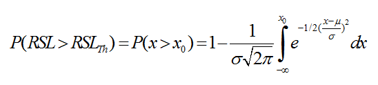
where
P = probability of rim coverage
x = receiver signal level (RSL)
x0 = receiver signal threshold (RSLTh)
μ = mean value representing the average received signal level
σ = standard deviation.
The standard deviation (μ) is estimated based on the probability distribution of RSL. For environments with severe attenuation, the number is between 6 and 10 dB. A value of 8 dB is used in the example shown in Table B.5-4. Only field testing can determine the exact value. In the example, the P(RSL>RSLTh) for 74% rim coverage is 0.65.
| Terms | Mine |
|---|---|
| Coverage objective | Mine coverage |
| Area coverage probability | 90% (n=4) |
| Rim coverage probability | 74% |
| Standard deviation (dB) | 8 dB |
| Fade margin (dB) | 0.65 x 8 = 5.2 dB |
B.5.6 Maximum Separation Distance
Given the minimum signal level required to minimize fading, the maximum coverage distance may be computed using the following:
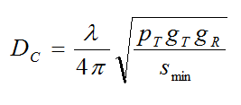
where
DC = maximum coverage distance (m)
pT = transmitter power (mW or W)
gT = transmitting antenna gain (numeric)
gR = receiving antenna gain (numeric)
λ = wavelength at the frequency of interest (m)
smin = minimum signal level required to minimize fading (mW or W)
Note that pT and smin must be in the same units. In addition, the coverage distance may be different if a propagation mode other than free space applies.
B.5.7 Passive Reflectors
Flat passive reflectors may be used in a mine to enhance the coverage into a crosscut. The reflector is arranged so that radiation from a transmitter reflects incident radiation into the crosscut. This configuration may have a lower path loss than a nonreflector configuration that is controlled by diffraction and scattering around the corner.
The effect of a passive reflector may be estimated by an approximate method where the reflector is modeled as if it is a receiving antenna [White 1975]. In this method, the gain of a passive reflector depends as follows on the frequency of the radio signal, the area of the reflector, and the included angle of the reflection:
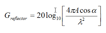
where
Greflector = passive reflector gain (dB)
A = reflector area (m2)
α = one-half the included angle of the reflection (degrees)
λ = wavelength of the radio signal (m)
Note that the reflector dimensions and wavelength must be expressed in the same units in the above equation. The gain in Equation (B-31) may be rewritten in convenient units as:
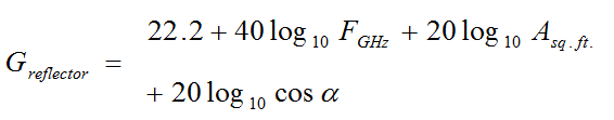
where all terms were previously defined.
Note that the area in the above equation is in square feet. For a link budget of a configuration that includes a passive reflector, first compute the propagation loss in dB along each leg of the complete path (i.e., transmitter-to-reflector and reflector-to-receiver). Parameter LP in Equation B-20 is then the sum of the propagation losses along the two legs minus the reflector gain Greflector.
The most typical use of a reflector in a mine would be to help redirect a portion of a radio signal's power in a mine entry down a crosscut (or vice versa). As an example, for a right-angle crosscut, the included angle of the reflection in this geometry is 90° (α is 45°) and the gain of a 4-square-foot reflector at 2.45 GHz would be 46.8 dB.
B.5.8 Node Placement: Percentage of Coverage Overlap
The percentage of coverage is given by taking the total distance between nodes and multiplying by 100% minus the desired mobile radio or phone unit overlap percentage to obtain the actual distance between nodes. For this tutorial, a desired mobile unit overlap of 25% is based on measurements of a typical cellular system. This approach ensures that the mobile unit has a 25% overlap between nodes. A higher overlapping area ensures reliable coverage but increases the cost. See Section B.5.9.3 for further discussion of coverage overlap.
B.5.9 Applications
B.5.9.1 Link Budget: Node-to-Node
The node-to-node link budget is calculated between two node units. The sample node-to-node link budget (Table B.5-5) calculates the maximum tolerable path loss between two adjacent nodes to obtain the maximum path distance between nodes that enables acceptable and reliable communications.
| Node-to-Node Link Parameters | Value | Basis | Source |
|---|---|---|---|
| Node Tx power (dBm) | 20.0 | a | Manufacturer |
| Node Tx power (W) | 0.1 | b | Manufacturer |
| Node Tx antenna gain (dBi) | 8.0 | c | Manufacturer |
| Node cable loss (dB) | 1.0 | d | Manufacturer |
| Node EIRP (dBm) | 27.0 | a+c-d | Section B.3.1 |
| Fade margin (FM) (dB) | 5.2 | e | Section B.5.5.2 |
| Node Rx antenna gain (dBi) | 8.0 | f | Manufacturer |
| Node cable loss (dB) | 1.0 | g | Manufacturer Section A.1.4 |
| kT (dBm/Hz) | -174 | h | Constant* Section B.5.2 |
| Node noise figure (dB) | i | Manufacturer | |
| Baud rate (dBHz) (i.e., 10 Mbps) | j | Manufacturer | |
| Average (Eb/No) (dB) | k | Section B.5.4.2 | |
| Node Rx Sensitivity (dBm) | -90 | RSL=k+j+i+h or given | Section B.5.4.2 or given |
| Maximum link path loss (dB) | 118 | l=a+c-d-e+f-g-RSL | B.4.2 |
| Frequency (GHz) | 2.4 | Manufacturer | |
| Maximum distance (m) | 400 | Section B.4.2 | Calculated |
| *kT = Boltzmann’s constant (1.38 * 10-23 joules/Δ°K) x room temperature (290°K) = -174 dBm/Hz | |||
B.5.9.2 Link Budget: Mobile-to-Node
The link budget calculates the maximum tolerable path loss for the reverse link and for the forward link, and then it takes the smaller of the two maximum loss values to determine the maximum distance of coverage.
The sample mobile-to-node reverse link budget (Table B.5-6) is calculated from the mobile unit to the node unit. The reverse link budget calculates the maximum tolerable path loss between the mobile unit and the node to obtain the maximum path distance that the node will cover to tolerate an acceptable and reliable communications.
| Reverse Link Parameters | Value | Basis | Source |
|---|---|---|---|
| Mobile Tx power (dBm) | 15 | a | Manufacturer |
| Mobile Tx power (W) | 0.0316 | b | Manufacturer |
| Mobile antenna gain (dBi) | 0.0 | c | Manufacturer |
| Mobile EIRP (dBm) | 15 | a+c | Section B.3.1 |
| Body loss (dB) | 2.0 | d | Manufacturer |
| Fade margin (FM) (dB) | 5.2 | e | Section B.5.5.2 |
| Node receiver antenna gain (dBi) | 8.0 | f | Manufacturer |
| Node cable loss (dB) | 1.0 | g | Manufacturer Section A.1.4 |
| kT (dBm/Hz) | -174 | h | Constant* Section B.5.2 |
| Node noise figure (dB) | i | Manufacturer | |
| Baud rate (dBHz) (i.e. 10 Mbps) | j | Manufacturer | |
| Mixed mobility average (Eb/N0) (dB) | k | 2 | |
| Node Rx sensitivity (dBm) | -90 | RSL=k+j+i+h or given |
Section B.5.4.2 or given |
| Maximum reverse link path loss (dB) | 104.8 | l=a+c-d-e+f-g-RSL | Section B.4.2 |
| Frequency (GHz) | 2.4 | Manufacturer | |
| Maximum distance (m) | 302 | Section B.4.2 | Calculated |
| *kT = Boltzmann's constant (1.38 * 10-23 joules/Δ°K) x room temperature (290°K) = -174 dBm/Hz | |||
The sample node-to-mobile link budget (Table B.5-7) is calculated from the node unit to the mobile unit. The forward link budget calculates the maximum tolerable path loss between the node and the mobile unit to obtain the maximum path distance that the node will cover to tolerate an acceptable and reliable communications.
| Forward Link Parameters | Value | Basis | Source |
|---|---|---|---|
| Node Tx power (dBm) | 20 | a | Manufacturer |
| Node Tx power (W) | 0.1 | b | Manufacturer |
| Node Tx antenna gain (dBi) | 8.0 | c | Manufacturer |
| Node cable loss (dB) | 1.0 | d | Manufacturer Section A.1.4 |
| Node EIRP (dBm) | 28 | a+c-d | Section B.3.1 |
| Fade margin (FM) (dB) | 5.2 | e | Section B.5.5.2 |
| MS Rx antenna gain (dBi) | 0.0 | f | Manufacturer |
| Body loss (dB) | 2.0 | g | Manufacturer |
| kT (dBm/Hz) | -174 | h | Constant* Section B.5.2 |
| Node noise figure (dB) | i | Manufacturer | |
| Baud rate (dBHz) (i.e. 10 Mbps) | j | Manufacturer | |
| Mixed mobility average (Eb/N0) (dB) | k | Section B.5.4.2 | |
| Mobile Rx sensitivity (dBm) | -90 | RSL=k+j+i+h or given |
Section B.5.4 or given |
| Maximum link path loss (dB) | 109.8 | l=a+c-d-e+f-g-RSL | Section B.4.2 |
| Frequency (GHz) | 2.4 | Manufacturer | |
| Maximum distance (m) | 339 | Section B.4.2 | Calculated |
| *kT = Boltzmann's constant (1.38 * 10-23 joules/Δ°K) x room temperature (290°K) = -174 dBm/Hz | |||
B.5.9.3 Node Placement: Percentage of Coverage Overlap
Near the edge of a node’s coverage, fading may cause reduced reliability of the communications link with mobile users. Designing the coverage of adjacent nodes to overlap increases the reliability of mobile connections in the edge region because it is less likely the link with both nodes will fade at the same time. For overlapping coverage, nodes are placed at a fraction (100% minus the desired mobile unit overlap percentage) of the maximum possible communication distance. For this tutorial, a mobile unit overlap of 25% is suggested based on measurements of a typical cellular system. This approach ensures that the mobile unit has a 25% overlap between nodes. A higher overlapping area increases reliability of coverage but also increases the cost.
From the example, the maximum distance between the mobile unit and the node is 302 m, therefore the distance between nodes is (2 x 302) x 0.75 = 453 m to ensure 75% rim coverage probability with a coverage overlap of 25%.
B.6 Electromagnetic Interference (EMI) Analysis
The objective of an EMI analysis is to compute the level of undesired power received by a possible victim receiver. It is similar to a link budget analysis, but all the losses and gains from a potential source system to the victim are cataloged.
This subsection describes the method for EMI analysis when an undesired signal from a transmitter is present at a receiver.
B.6.1 Frequency Coincidence
Major EMI interactions are based on the following cases of frequency coincidence between a transmitter and a victim receiver:
- Co-channel (CC) interference occurs when a transmitter and receiver share the same frequency band and their tuned frequencies are identical or very close to each other. Energy from the transmitter emission spectrum overlaps the receiver’s passband.
- Adjacent-channel (AC) interference occurs when a transmitter and receiver share the same frequency band and their tuned frequencies are not identical but close to each other. Energy contained in the emission spectrum sidebands overlaps the receiver selectivity.
- Adjacent-band (AB) interference occurs when a transmitter and receiver are in different frequency bands and their tuned frequencies are close to each other. Energy contained in the emission spectrum sidebands overlaps the sidebands of the receiver selectivity.
- Harmonic (HR) interference occurs when a transmitter and receiver are generally in different frequency bands and the frequency of a transmitter harmonic is identical or very close to the receiver’s tuned frequency. The undesired energy is at an integer multiple of the transmitter’s fundamental frequency.
The CC, AC, and AB cases tend to be of most concern because of the high power involved at the fundamental frequency. HR cases are of less importance because of the reduced transmitter power and any antenna out-of-band (OOB) effects, but are still a concern.
The frequency coincidence for the four frequency coincidence cases may be determined by comparing the tuning bands of the two subsystems. Frequency coincidence definitions are given below.
B.6.2 Undesired Received Power
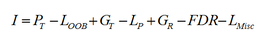
When two antennas are in the far-field of each other, the level of undesired received power may be computed using the following equation:
where
I = received undesired signal power (dBm)
PT = transmitter power at the fundamental frequency (dBm)
LOOB = correction factor to account for an interaction at an OOB frequency (dB). For a harmonic interaction, LOOB is applied to the transmitter power.
GT = transmit antenna gain (dBi). GT is the gain in the direction of the propagation ray path.
LP = total propagation loss between antennas (dB). LP is evaluated at the receive frequency, and includes any additional losses (diffraction, reflection, absorption, etc.) along the ray path between antennas.
GR = receive antenna gain (dBi). GR is the gain in the direction of the propagation ray path.
FDR = frequency-dependent rejection (FDR) (dB). See Section B.6.3 for a description of this parameter.
Lmisc = total of any additional miscellaneous losses (dB). Lmisc could include such terms as antenna loss at an OOB frequency, filtering loss, or miscellaneous system loss.
The above equation is the general equation to be used for EMI analysis. Because the undesired signal may be at a frequency different than the tuned frequency for the receiver, the above equation includes terms to account for OOB effects.
B.6.3 Frequency-Dependent Rejection (FDR)
FDR consists of two components. The on-tune rejection (OTR) component is due to the difference in bandwidths (BW) between the selectivity and the emission spectrum, assuming that the receiver and transmitter are tuned to the same frequency (i.e., the difference in frequencies, Δf, is zero). The off-frequency rejection (OFR) component is due to any off-tuning between the transfer functions representing the selectivity and the emission spectrum. FDR is related to OTR and OFR by the following:
where FDR, OTR, and OFR are all in dB.
When the BW of the receiver selectivity is greater than or equal to the BW of the emission spectrum, the receiver accepts all of the power of the undesired signal. Hence, the OTR term is zero for this case. On the other hand, when the BW of the selectivity is less than the BW of the emission spectrum, the receiver accepts only a portion of the power, and the magnitude of the OTR term is greater than zero. The OTR is independent of Δf.
The OFR term is a function of Δf. The OFR term is zero when the receiver and the transmitter are tuned to the same frequency and its magnitude increases as Δf increases.
An approximate, conservative method, referred to as Quick FDR [17], may be used for the evaluation of FDR. Inputs to the calculation of Quick FDR are the -3 dB BW of the IF stage selectivity and the -3 dB BW of the emissions spectrum. Other inputs are the rolloff of the selectivity and the spectrum. Each rolloff defines the rate of attenuation with respect to frequency. Rolloff values, in dB per decade of frequency, are computed from the IF selectivity and emissions spectrum data. In the absence of data, typical rolloffs are -40 dB per decade for the transmitter and -80 dB per decade for the receiver.
B.6.4 Interference-to-Noise Ratio
The interference-to-noise power ratio (INR) is useful in undesired-signal analysis and may be found as follows:
where
INR = available interference-to-noise power ratio (dB)
I = undesired signal power (dBm)
N = receiver effective noise power level, including any external noise (dBm).
When I is a measurement or prediction of the available undesired signal level under certain conditions, then INR is the available INR. As for the desired-signal analysis, N is the effective noise power in the -3 dB passband of the receiver’s narrowest IF stage.
B.6.5 Undesired Signal Power Threshold
The undesired signal power threshold is the maximum allowable received power that a receiver can accept without degradation of its performance. The undesired signal power threshold, IT, may be computed using the following:
where
IT = undesired signal power threshold(dBm)
N = receiver effective noise power level, including any external noise (dBm)
INRT = interference-to-noise threshold (dB)
Note that the INRT in the above equation is a threshold INR, which is different than the available INR mentioned in the previous subsection B.6.4. A negative value of INRT is usually selected so that the threshold is below the receiver effective noise level. A typical value is -6 dB.
As a numerical example, suppose that the effective noise level, N, in a receiver’s IF bandwidth is -120 dBm. Also, suppose that the interference threshold, INRT, is -6 dB. The maximum allowable received power, IT, to avoid receiver degradation would then be -126 dBm.
B.6.6 Interference Margin
A parameter referred to as the interference margin or EMI margin may be computed to quantify the level of EMI. The EMI margin may be computed using the following:
where
M = EMI margin (dB)
I = received undesired power (dBm)
IT = undesired signal power threshold (dBm)
The EMI margin may be interpreted as the additional loss that would be required to reduce the undesired received power to a level below the threshold. Continuing the example from the previous subsection, if I is computed to be -100 dBm, the EMI margin would be 26 dB.
B.6.7 Required Frequency Separation (RFS)
The required frequency separation (RFS) may be computed using a loss, LRFS, that is similar to the EMI margin, but with frequency dependent rejection (FDR) excluded. LRFS would be the loss required for the received power to be equal to the receiver threshold given an off-tuning between the transmitter and the receiver. The LRFS may be computed using the following equation:
where all terms were defined previously. Given a value for LRFS, the RFS may be evaluated using multiple calls to Quick FDR where a search algorithm is employed to determine the frequency difference that would result in a loss approximately equal to LRFS.
B.7 Hazards of Electromagnetic Radiation
One of the concerns of introducing wireless systems in a coal mine is potentially hazardous EM radiation from transmitting systems. The concerns include hazards of EM radiation to miners. Higher levels of EM radiation can have the potential of detonating blasting caps and can even cause a methane or coal dust explosion under certain optimal conditions.
B.7.1 Threshold Levels
B.7.1.1 Personnel
For hazards of electromagnetic radiation to personnel (HERP), levels of maximum permissible exposure (MPE) were obtained [IEEE 2006 and CFR 47]. Certain of the MPE levels of CFR 47 were determined to be lower than those of IEEE C95.1 [IEEE 2006), and were used in the analyses. IEEE C95.1 notes that the exposure limits in the frequency range from 100 MHz to 1500 MHz are generally based on guidelines from CFR 47§1.1310.
Exposure of personnel to hazardous radiation is tiered based upon frequency. All of the following assume an external, sinusoidal-based, electromagnetic field in a controlled environment. A controlled environment is defined as "an area that is accessible to those who are aware of the potential for exposure as a concomitant of employment, to individuals cognizant of exposure and potential adverse effects, or where exposure is the incidental result of passage through areas posted with warnings, or where the environment is not accessible to the general public and those individuals having access are aware of the potential for adverse effects." [IEC 2007]
The following are from Table 1, Limits for Occupational/Controlled Exposures [CFR 47 Part 1 Paragraph 1.1310 2007a]:
0.3-3.0 MHz
RMS electric field strength should not exceed 614 V/m averaged over 6 minutes.
RMS magnetic field strength should not exceed 1.63 A/m averaged over 6 minutes.
Note: For frequencies below 30 MHz, IEEE Std C95.1-2005 mandates that both the E and the H fields be computed. The reason for this is not indicated, but presumably it is to account for possible near-field effects. For any systems with frequencies in the range of 0.3 to 3.0 MHz, both fields were computed.
3.0-30 MHz
The root-mean-square (rms) electric field strength should not exceed 1842/fMHz V/m averaged over 6 minutes, where fMHz is the frequency in MHz.
The rms magnetic field strength should not exceed 4.89/fMHz A/m averaged over 6 minutes.
Note: For frequencies below 30 MHz, Stallings [2007] mandates that both the E- and the H-fields be computed. For any systems with frequencies in the range of 0.3 to 3.0 MHz, both fields were computed.
30-300 MHz
RMS electric field strength should not exceed 61.4 V/m averaged over 6 minutes.
RMS magnetic field strength should not exceed 0.163 A/m averaged over 6 minutes.
300-1500 MHz
Average power density should not exceed fMHz/300 milliwatts per square centimeter (mW/cm2) averaged over 6 minutes.
1.5-100 GHz
Average power density should not exceed 5 mW/cm2 averaged over 6 minutes.
B.7.1.2 Blasting Caps
The applicable threshold for a blasting cap is its no-fire level of power. The threshold level was obtained from IEEE C95.4 [IEEE 2002a].
The specification or measured no-fire threshold of the blasting cap should be used, if known. If unknown, the typical no-fire threshold, 40 mW (16 dBm) average power, should be used.
B.7.1.3 Explosive Atmospheres
Applicable thresholds for an explosive atmosphere were obtained from IEC 60079-0 [IEC 2007]. IEC 60079-0 lists thresholds of radio frequency devices operating over a frequency range from 9 kHz to 60 GHz. The thresholds are presented for five different groups representing different environments. Underground coal mines fall under Group 1.
The thresholds are defined with respect to a “thermal initiation time.” The thermal initiation time is the time during which energy deposited by a spark accumulates in a small volume of gas around it without significant thermal dissipation. For times shorter than the thermal initiation time, whether or not ignition occurs depends on the total energy deposited by the spark. For times longer than the thermal initiation time, whether or not ignition occurs depends on the effective radiated power.
For systems capable of continuous transmissions, the threshold is given in terms of the “threshold power” in watts. This threshold also applies to systems capable of pulsed transmissions, where the pulse width exceeds the thermal initiation time. For Group 1, Table 4 of IEC 60079-0 [IEC 2007] defines the transmitter threshold power level to be 6 watts, and the thermal initiation time to be 200 μs.
Threshold power is defined to be the effective output power of the transmitter multiplied by the antenna gain. In equation form, this is expressed in the follow equation:
where
pthr = transmitter’s threshold power (W)
pT = transmitter power at the input to the antenna (W)
gT = maximum far-field transmit antenna gain (numeric)
Maximum transmitter power and maximum far-field transmit antenna gain were used in computing the threshold power. An antenna's gain value is most often relative to an isotropic antenna, a theoretical concept where radiation is equal in all directions. From the above, the threshold power is then identical to the EIRP.
For systems with a pulsed waveform, where the pulse width is less than the thermal initiation time (200 μs), the standard is defined in terms of the maximum threshold energy of the pulsed transmission in μJ. Table 5 of IEC 60079-0[IEC 2007] defines the maximum threshold energy level to be 1500 μJ for Group 1.
The threshold energy may be computed using the following:
where
wthr = transmitter’s threshold energy (μJ)
τ = transmitter's pulse width (μs)
and other terms were defined previously.
B.7.2 Required Separation Distances (RSD), VHF and Higher Frequency Bands
For systems having tuned frequencies in the VHF band and above, required separation distances (RSDs) were computed using transmitter power, far-field antenna gain, and free-space equations. Equations for computing the RSDs are given in the following subsections B.7.2.1 through B.7.2.4. Although antenna radiation is strongest in the near-field region, near-field antenna effects were not considered in the calculation of the RSDs because of time constraints and a lack of detailed antenna data. Nevertheless, for safety reasons, a field/power density multiplier was included in the calculation of the RSDs (see below).
For systems having tuned frequencies in the medium frequency (MF) band, far-field antenna gain and free-space conditions are not applicable. Order-of-magnitude values of the fields and received power values were estimated using data from a manufacturer.
B.7.2.1 Power Density Threshold
The average power density (s) incident on a point may be computed using the following equation [Balanis 2005]:
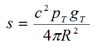
where
s = average power density (W/m2)
c = constant multiplier to account for reflections
pT = transmitter power (W)
gT = far-field transmit antenna gain (numeric)
R = distance from the antenna to the point of interest (m)
In the analyses, maximum transmitter power and maximum far-field antenna gain were used. If pT and gT are maximum values for the system, then s is the maximum average power density.
As indicated, c is a multiplier that was included to account for reflections. For one perfect reflection, the constant c would have a value of 2.0, indicating that twice the field would be incident on some point in space. From Equation B-41, four times the power density would be incident. Similarly, for two perfect reflections, constant c would have a value of 3.0, indicating that three times the field, or nine times the power density, would be incident on the point.
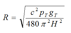
For an MPE expressed in terms of threshold power density s, the RSD may be computed by solving Equation B-41 for R:
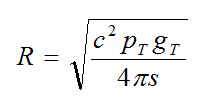
where
R = RSD (m)
s = threshold power density (W/m2)
and all other terms have been defined previously.
B.7.2.2 Electric Field Threshold
For an MPE expressed in terms of electric field strength E, the electric field strength may be related to the power density as follows [Kraus 1992]:
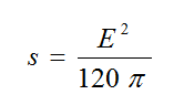
where E is the RMS electric field strength in volts/m and s was defined previously.
The RSD may be computed by substituting Equation B-43 into Equation B-41 and simplifying:
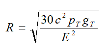
where E is the threshold RMS electric field strength in V/m and all other terms have been defined previously.
B.7.2.3 Magnetic Field Threshold
For an MPE expressed in terms of threshold magnetic field strength H, the magnetic field strength may be related to the threshold power density as follows [Kraus 1992]:
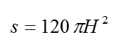
where H is the rms magnetic field strength in amperes/m and s was defined previously.
The RSD may be computed by substituting Equation B-45 into Equation B-41 and simplifying:
where H is the threshold rms magnetic field strength in A/m and all other terms have been defined previously.
B.7.2.4 Received Power Threshold
The power received by an antenna, or a wire acting as an antenna may be computed using the following Equation [Balanis 2005]:
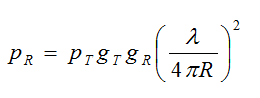
where
pR = received power at the output of the receiving antenna (W)
pT = transmitter power (W)
gT = transmitting antenna gain (dBm)
gR = receiving antenna gain (dBm)
λ = wavelength at the frequency of interest (m)
R = distance between antennas (m)
In the analyses, maximum transmitter power and maximum far-field antenna gains were used, so that pR is the maximum average received power.
In the case of a blasting cap, it was assumed that a wire or a pair of wires connected to the cap is acting incidentally as a "receiving antenna." The wire or wires were assumed to be a half-wavelength long at the frequency of the transmitter, so the numeric gain would be 1.64 [Balanis 2005].
For a threshold, pthr, expressed in terms of received power, the RSD may be computed by substituting pthr for pR and solving Equation B-47 for R:
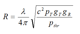
where R is the RSD in m.
- Above-the-Earth Field Contours for a Dipole Buried in a Homogeneous Half-Space
- Medium-Frequency Propagation in Coal Mines
- Mine Communications and Tracking Glossary
- Mine Communications Engineering and Compatibility Guidelines
- Propagation of EM Signals in Underground Mines
- Technology News 544 - New Measurement Tool to Validate Wireless Communications and Tracking Radio Signal Coverage in Mines
- Through-The-Earth Wireless Real-Time Two-Way Voice Communications
- U.S. Bureau of Mines New Developments in Mine Communications
- Underground Mine Communications
- Wireless Mesh Mine Communication System