Scenario Modeling Methods - COVID-19

COVID-19 scenario modeling overview

Scenario models are a type of disease model that explore medium- to long-term hypothetical outcomes under different assumptions about the future. Unlike forecasts produced for the short-term future, scenario models do not aim to predict the future; instead, they allow us to explore "what-if" hypothetical situations. By exploring potential scenarios, decision-makers can better prepare and plan for an uncertain future. Our Behind the Model shares more about how scenario modeling can be used to inform decision-making. In this document, we focus on scenario models produced by CFA, which are submitted to the Scenario Modeling Hub and used in CFA's Respiratory Season Outlooks. Research or operational questions determine the focus for each round of scenario modeling from the Scenario Modeling Hub; previous rounds have focused on the impact of changes in behavior, vaccination, and the introduction of new variants. Specific scenarios defined for the Respiratory Season Outlooks also vary by the respiratory season, but have focused on peak timing and size and variant emergence.

We project COVID-19 dynamics under different scenarios using a transmission model with a compartmental modeling structure that takes into account population age structure, infection history, vaccination history, immunity waning status, and SARS-CoV-2 variants. Immunity is determined by immunogenic events (infections and vaccinations) and time since the most recent event. Protection against infection is variant-specific: past infection with a more similar variant, or vaccination with a better-matched vaccine, provides a higher level of protection against the challenging variant. The model uses mathematical equations, implemented in computer code, to describe how groups move between compartments (e.g., from uninfected to infected or from unvaccinated to vaccinated).

Detailed model structure

The COVID-19 model used for the 2025–2026 Outlook is a Susceptible, Exposed, Infectious, Susceptible (SEIS) model, which models the movement between the population states Susceptible, Exposed, Infectious, and back to Susceptible. Each compartment is stratified by several factors, or dimensions: age group, vaccination status, infecting variant, and immunity levels, which wane over time and are boosted by vaccination and infection. The categories within each dimension (e.g., not vaccinated, one dose of vaccination, etc.) are shown in Table 1.

View Larger

Show More

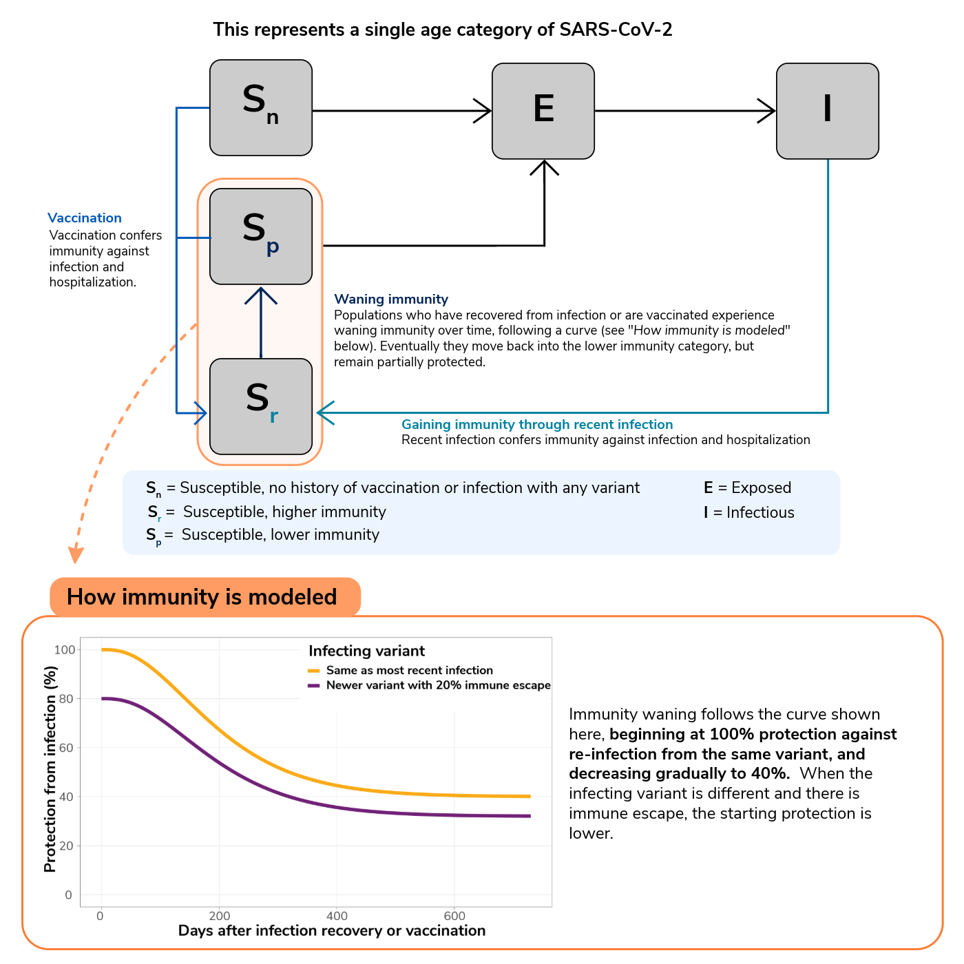
To illustrate this structure, let's consider a single age group and SARS-CoV-2 variant (Figure 1). Populations who are susceptible to infection and have no vaccination or recent infection (and therefore immunity) are treated as a single group (S_n). When they are infected but not yet infectious, they move to the exposed compartment (E). When they become infectious, they move into the infectious compartment (I). Following a period of infectiousness, they then return to being susceptible but move to a higher immunity compartment due to their recent infection (S_r). They then could be re-infected and move into the exposed compartment or, in the absence of a new infection and as immunity wanes, they will return to the lower-immunity category but retain partial immunity (S_p). This immunity category is not specific to vaccination or past infection. This structure occurs for each age group and SARS-CoV-2 variant. These structures are interconnected: people across different age groups are mixing, allowing for transmission across age-groups.

Newly introduced variants have immune-escape properties that may allow them to spread in a population that is highly immune to previous variants. If the infecting variant is different than the variant that populations were vaccinated against or recently infected with, flow may still occur from S_r to E. The introduction of a particular SARS-CoV-2 variant is determined by parameters defining the introduction time. These parameters are estimated for historical variants, and the distributions of those estimates are used to inform scenarios for future potential variants.

Immunity

Upon recovery or vaccination, people are placed at the high immunity status regardless of their previous immunity status. By representing immunity as people “flowing” between these high and low states of partial protection, we approximate population-level immunity that changes smoothly over time (Figure 1 and 2). For re-exposures to the same variant that caused the most recent infection, we assume high immunity status confers 100% protection from infection; this protection wanes to 40% for low immunity status. The half-life of this protection, or amount of time for people to decrease from 100% protection to 70%, is approximately 188 days. When challenged with newer variants with, for example, 20% immune escape, the high immunity status confers only 80% protection from infection and eventually wanes to 32% protection. These assumptions imply an immunity waning profile as shown in the bottom panel of Figure 1.

Hospitalization rate modeling

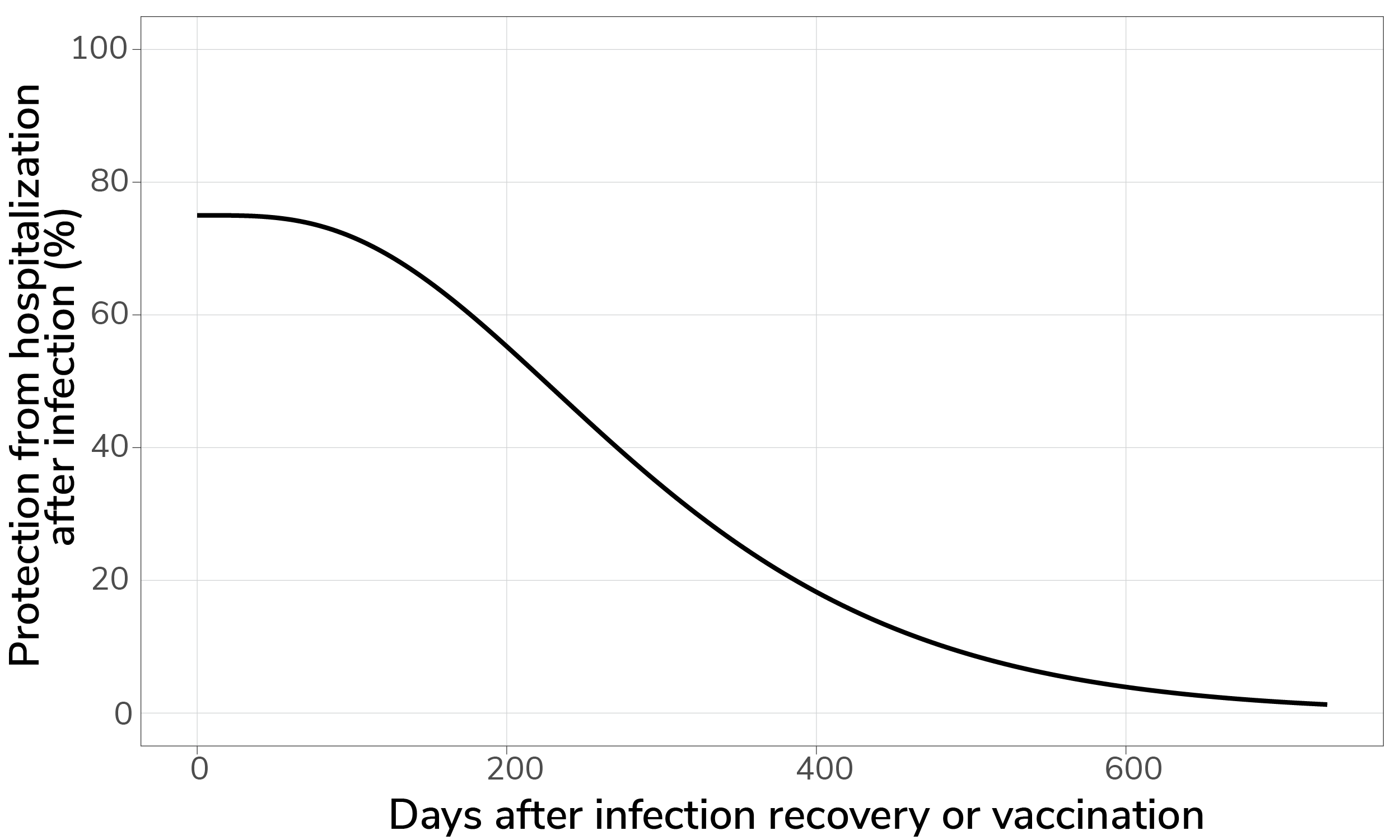
Our model estimates hospitalizations from infections using infection-hospitalization ratios (IHRs). These ratios represent the proportion of infections that result in reported hospitalizations. In our model, infection-hospitalization ratios vary by age group and are influenced by immunity (as discussed in previous section). We assume that people who have recovered from a past infection or received vaccination have a reduced IHR when reinfected and that this benefit is stronger when the immunizing event was recent. This protection factor is estimated by the model to start around 75% and follows the same waning profile as protection from infection (Figure 2). Because the primary effect of vaccination in the model is refreshing existing immunity, vaccine effectiveness against hospitalization is an output of the model. Our model has an implied population-wide relative vaccine effectiveness against hospitalization of 40%, on average, over the 2025-26 respiratory virus season.

View Larger

We also assume that more recent variants, starting with JN.1 (Winter 2023), are associated with a lower IHR than variants prior to JN.1. We multiply the estimated hospitalization risks to modeled daily infections to generate daily hospitalizations by age group, using a one-week lag between infections and hospitalization. These daily estimates are then aggregated into weekly totals to generate state-level hospitalization projections across the United States. This approach does not consider hospital capacity or occupancy and assumes that hospitalization does not have a substantial effect on transmission.

Parameter fitting

The COVID-19 model is calibrated to hospitalization data for each U.S. state. For the 2025-2026 Respiratory Disease Season Outlook, we used National Hospital Surveillance Network hospitalization rate data for two states and projected hospitalization rates inferred from National Syndromic Surveillance Program emergency department visit data for 48 states (due to previous gaps in hospitalization data reporting from NHSN). To infer hospitalization rates from NSSP emergency department visit data, weekly data from April 20, 2023 through April 20, 2024, were used to train four candidate models: a linear model, a linear model with a one-week lag, a generalized additive model, and a generalized additive model with a one-week lag. The best-fitting model was selected separately for each state and age group and used to generate NSSP-inferred hospitalization estimates. Model fitting was carried out by calibrating model-produced hospitalization counts to observed hospitalization counts using an SVI (Stochastic Variational Inference) approach. See Table 2 for key parameters, values, and any references for fixed values.

Scenarios

The following two scenarios were modeled for the Respiratory Outlook 2025-26:

1. No emergence of a new variant with significant immune-escape properties: Assumes that no variant will emerge that significantly evades the population's immunity.
2. Emergence of a variant with moderate immune-escape properties in November: People in the model experience a small risk of exposure to the new variant from an outside source that increases gradually over two weeks, peaks on November 1, and then decreases over two weeks. This exposure risk seeds infections that can then propagate via transmission within the population. We assumed that this variant had similar properties to the variants that were dominant during the summer 2024 and winter 2024-25 waves.

Both scenarios assumed that only people 65+ and those with underlying health conditions would receive a COVID-19 vaccine in the 2025-2026 season. In the model, the 65+ age group received vaccines at the same rate as in 2024-2025. A proportion of 18- to 64-year-olds equivalent to the proportion of the population with relevant underlying conditions ("high-risk" groups) also received vaccination at the same rate as in 2024-2025. We also assumed vaccine effectiveness against infection was the same as in 2024-2025. In the scenario in which a November variant with moderate immune escape properties emerges, variant-specific parameters were defined by sampling from the posterior distributions of variant-specific parameters for the last two important variants (the posterior distributions for immune protection in the previous two waves had mean estimates of 72.4% (SD 4.1%) and 83.1% (SD 2.6%), respectively). We then combined these samples, fit a new multi-variate Gaussian distribution to the combined samples, and then sampled from the new distribution to produce the parameters for the new variant. We produced forward projections for each state and scenario and then aggregated the state-level output to produce national projections.

Resources

1. Behind the Model: How Scenario Modeling Can Inform Public Health Decision-Making | CFA: Behind the Model | CDC
2. COVID-19 Scenario Modeling Hub
3. GitHub repository for the Underlying Ordinary Differential Equation Modeling Framework