At a glance
- This appendix provides guidance on epidemiologic and descriptive statistical methods to assess cancer occurrences.
- The standardized incidence ratio (SIR) is often used to assess if there is an excess number of cancer cases.
- Alpha, beta, and statistical power relate to the types of errors that can occur during hypothesis testing.
Overview
This section provides general guidance regarding epidemiologic and descriptive statistical methods most commonly used to assess occurrences of cancer. Frequencies, proportions, rates, and other descriptive statistics are useful first steps in evaluating the suspected unusual pattern of cancer. These statistics can be calculated by geographical location (e.g., census tracts) and by demographic variables such as age category, race, ethnicity, and sex. Comparisons can then be made across different stratifications using statistical summaries such as ratios.
Standardized incidence ratio
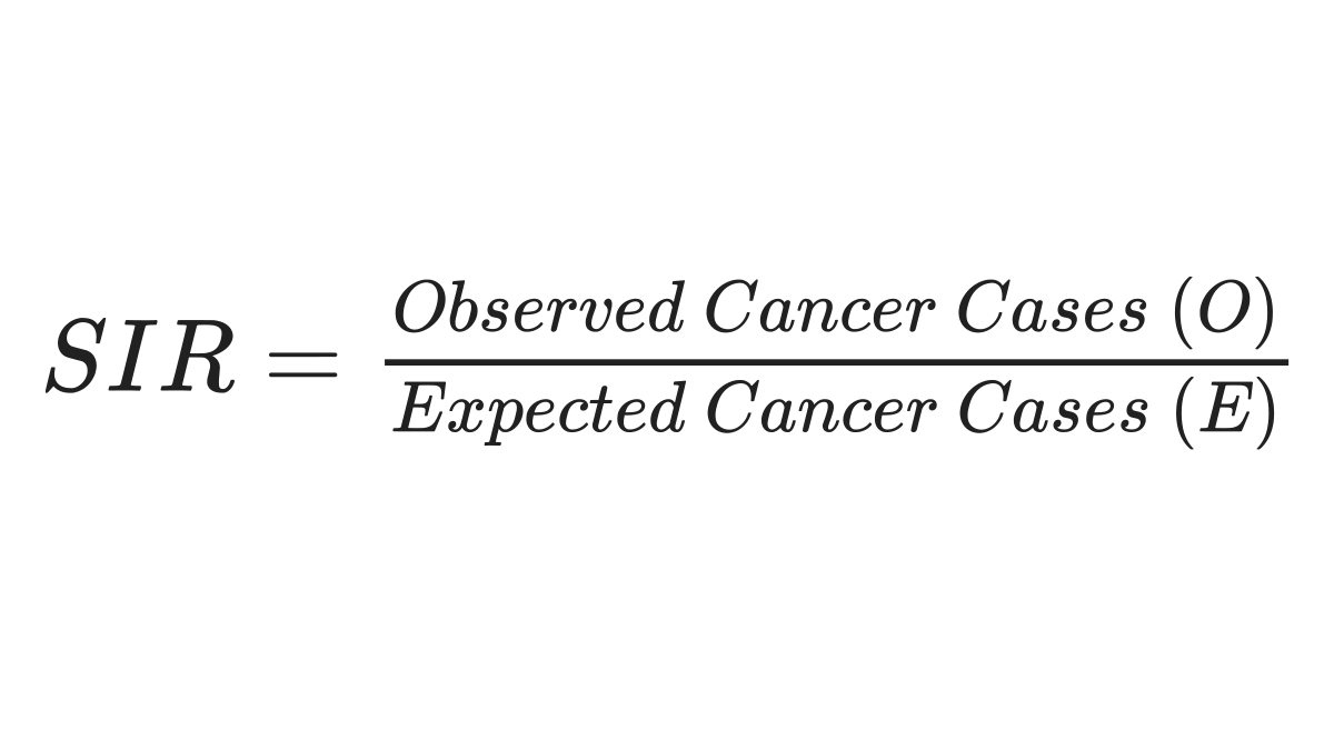
The standardized incidence ratio (SIR) is often used to assess whether there is an excess number of cancer cases, considering what is “expected” to occur within an area over time given existing knowledge of the type of cancer and the local population at risk. The SIR is a ratio of the number of observed cancer cases in the study population compared to the number that would be expected if the study population experienced the same cancer rates as a selected reference population. Typically, the state as a whole is used as a reference population. The equation is as follows:
Adjusting for factors
The SIR can be adjusted for factors such as age, sex, race, or ethnicity, but it is most commonly adjusted for differences in age between two populations. In cancer analyses, adjusting for age is important because age is a risk factor for many cancers, and the population in an area of interest could be, on average, younger or older than the reference population12. In these instances, comparing the crude counts or rates would present a biased comparison.
For more guidance, this measure is explained in many epidemiologic textbooks, sometimes under standardized mortality ratio, which uses the same method but measures mortality instead of incidence rates3456789. Two ways are generally used to adjust via standardization, an indirect and a direct method. An example of one method is shown below, but a discussion of other methods is provided in several epidemiologic textbooks3 and reference manuals10.
An example is provided in the table below, adjusting for age groups. The second column, denoted with an "O," is the observed number of cases in the area of interest, which in this example is a particular county within the state. The third column shows the population totals for each age group within the county of interest, designated as "A." The state age-specific cancer rates are shown in the fourth column, denoted as "B." To get the expected number of cases in the fifth column, A and B must be multiplied for each row. The total observed cases and the total expected cases are then summarized.
| Age Group
|
Observed Number of Cases in County*
(O) |
County of Interest Population
(A) |
State Age-Specific Cancer Rate†
(B) |
Expected Cancer Cases
(A x B= E) |
|---|---|---|---|---|
| 40-49 | 50 | 20,000 | 0.001 | 20 |
| 50-59 | 150 | 23,000 | 0.007 | 161 |
| 60-69 | 200 | 25,000 | 0.010 | 250 |
| 70+ | 250 | 15,000 | 0.015 | 225 |
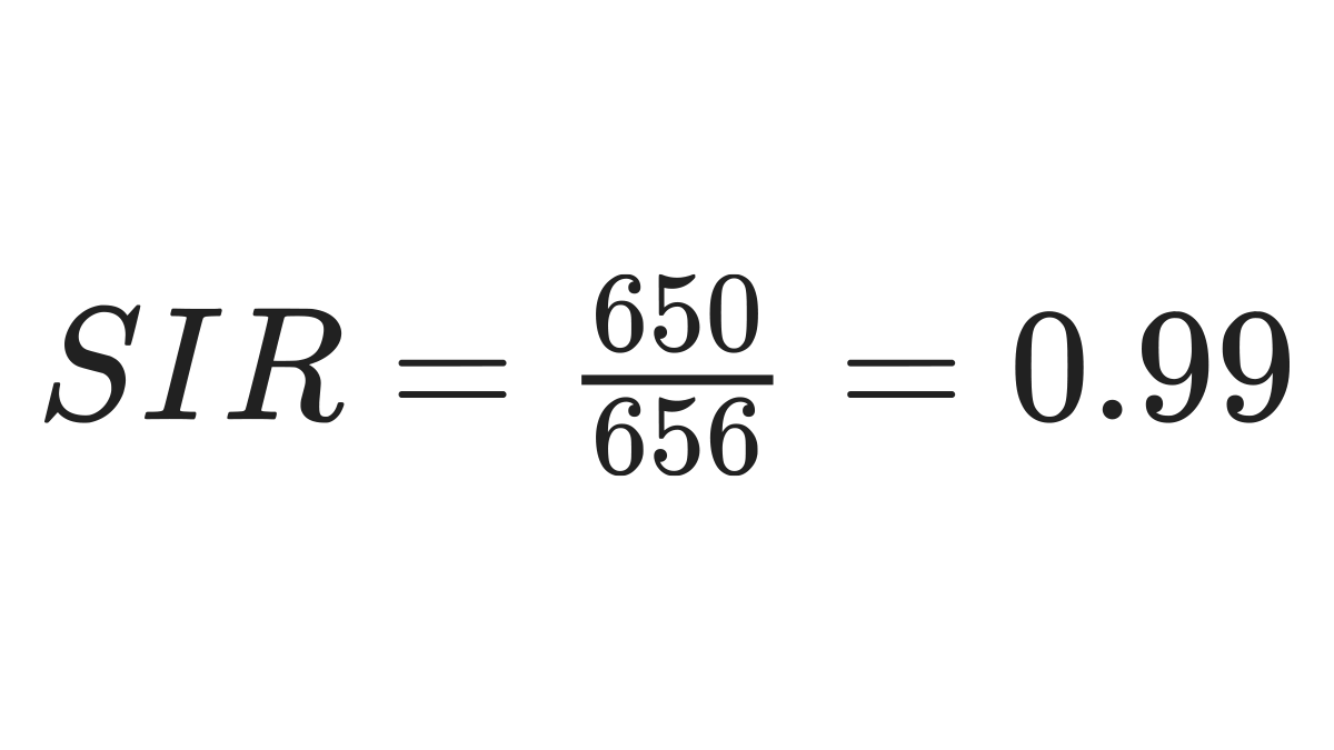
| Total | 650 | - | - | 656 |
*Number of cases in a specified time frame.
† Number of cases in the state divided by the state population for the specified time frame. Rates are typically expressed per 100,000 or 1,000,000 population.
The number of observed cancer cases can then be compared to the expected. The SIR is calculated using the formula below.
Confidence intervals
A confidence interval (CI) is one of the most important statistics to be calculated, as it helps to provide understanding of both statistical significance and precision of the estimate. The narrower the confidence interval, the more precise the estimate4 .
A common way of calculating confidence intervals for the SIR is shown below 4:
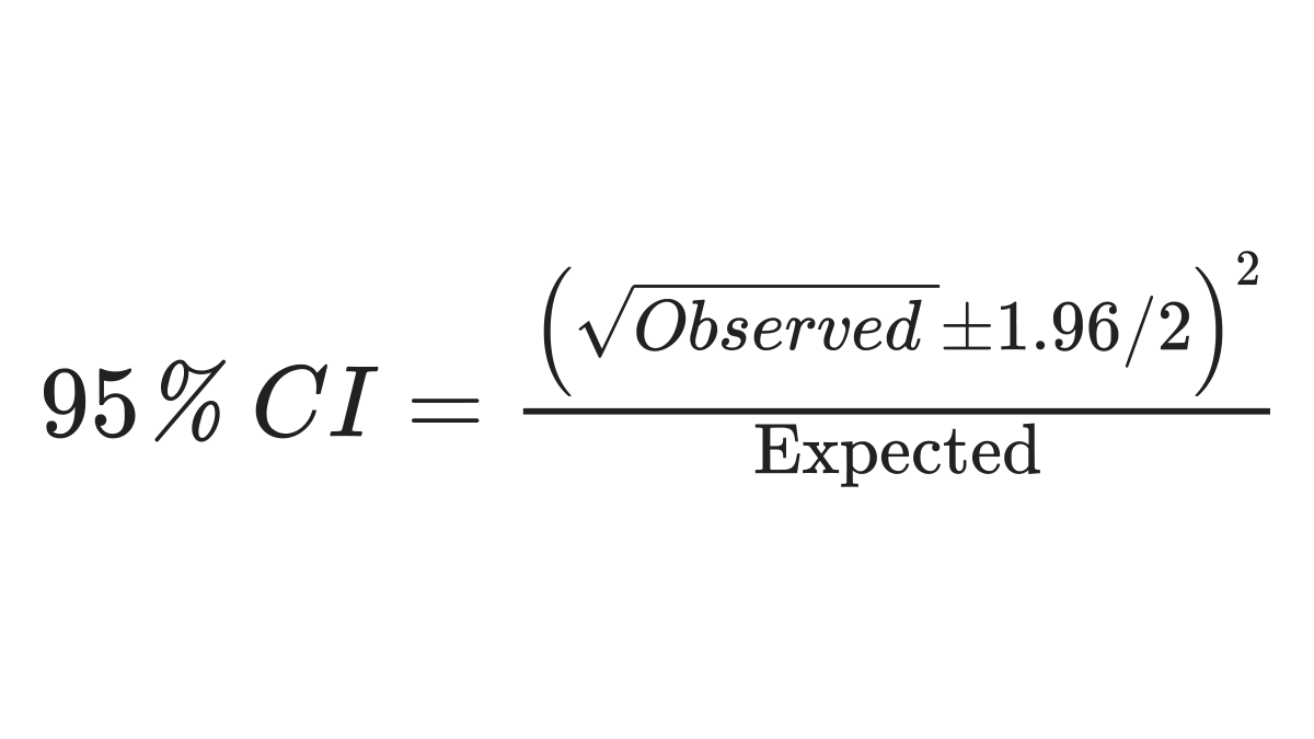
Using the example above produces this result:
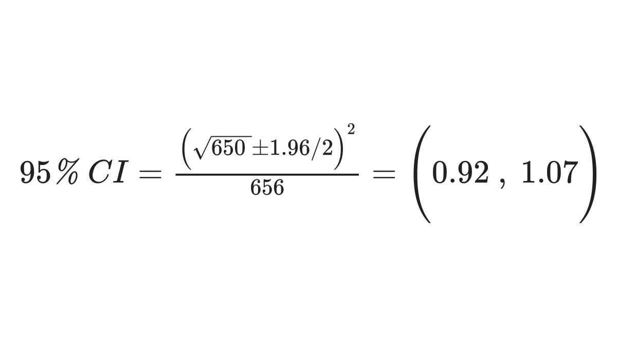
If the confidence interval for the SIR includes 1.0, the SIR is not considered statistically significant. However, there are many considerations when using the SIR. Because the statistics can be impacted by small case counts, or the proportion of the population within an area of interest, and other factors, the significance of the SIR should not be used as the sole metric to determine further assessment in the investigation of unusual patterns of cancer. Additionally, in instances of a small sample, exact statistical methods, which are directly calculated from data probabilities such as a chi-square or Fisher’s exact test, can be considered. These calculations can be performed using software such as R, Microsoft Excel, SAS, and STATA9. A few additional topics regarding the SIR are summarized below.
Reference population
Decisions about the reference population should be made prior to calculating the SIR. The reference population used for the SIR could be people in the surrounding census tracts, other counties in the state, or the entire state. Selecting the appropriate reference population is dependent upon the hypothesis being tested and should be large enough to provide relatively stable reference rates. One issue to consider is the size of the study population relative to the reference population. If the study population is small relative to the overall state population, including the study population in the reference population calculation will not yield substantially different results. However, excluding the study population from the reference population may reduce bias. If the reference population is smaller than the state as a whole (such as another county), the reference population should be “similar” to the study population in terms of factors that could be confounders (like age distribution, socioeconomic status and environmental exposures other than the exposure of interest). However, the reference population should not be selected to be similar to the study population in terms of the exposure of interest. Appropriate comparisons may also better address issues of health equity. Ultimately, careful consideration of the refence population is necessary since the choice can impact appropriate interpretation of findings and can introduce biases resulting in a decrease in estimate precision.
Limitations and further considerations for the SIR
One difficulty in community cancer investigations is that the population under study is generally a community or part of a community, leading to a relatively small number of individuals comprising the total population (e.g., small denominator for rate calculations). Small denominators frequently yield wide confidence intervals, meaning that estimates like the SIR may be imprecise5. Other methods, such as qualitative analyses or geospatial/spatial statistics methods, can provide further examination of the cancer and area of concern to better discern associations. Further epidemiologic studies may help calculate other statistics, such as logistic regression or Poisson regression. These methods are described in Appendix B. Other resources can provide additional guidance on use of p-values, confidence intervals, and statistical tests3491112.
Alpha, beta, and statistical power
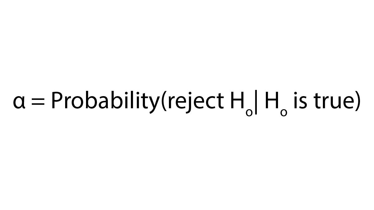
Another important consideration in community cancer investigations is the types of errors that can occur during hypothesis testing and the related alpha, beta, and statistical power for the investigation. A type I error occurs when the null hypothesis (Ho) is rejected but actually true (e.g., concluding that there is a difference in cancer rates between the study population and the reference population when there is actually no difference). The probability of a type I error is often referred to as alpha or α13.
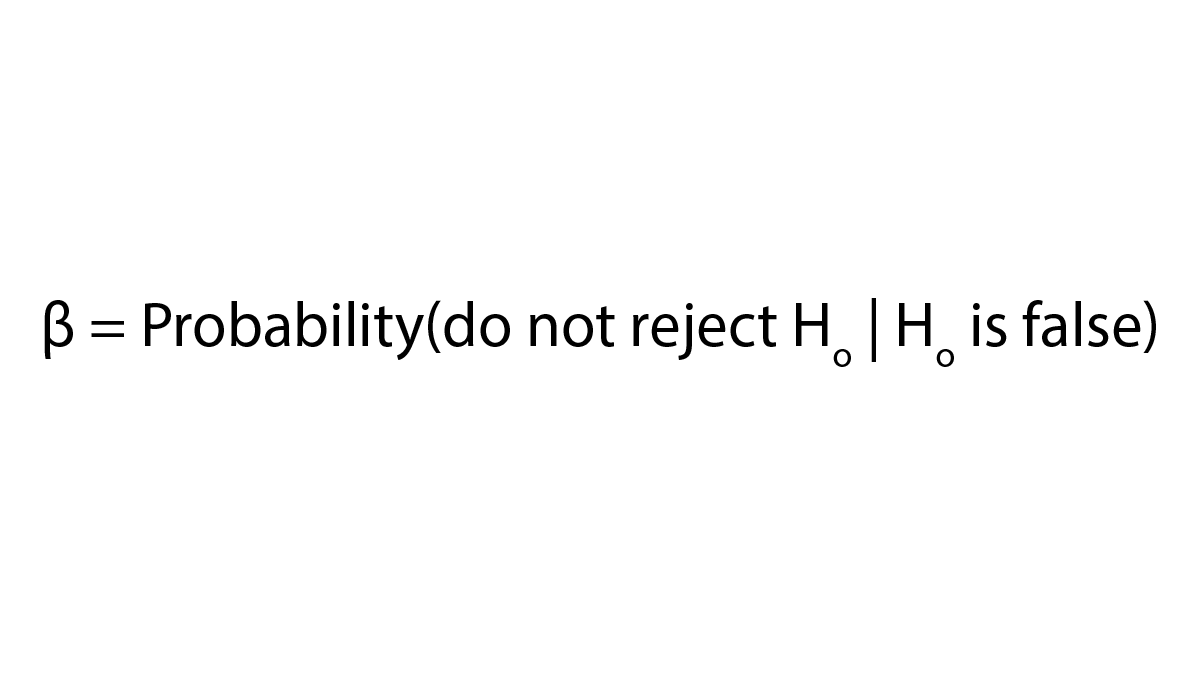
A type II error occurs when the null hypothesis is not rejected and it should have been (e.g., concluding that there is no difference in cancer rates when there actually is a difference). The probability of a type II error is often referred to as beta or β.
Power is the probability of rejecting the null hypothesis when the null hypothesis is actually false (e.g., concluding there is a difference in cancer rates between the study population and reference population when there actually is a difference). Power is equal to 1-beta. Power is related to the sample size of the study—the larger the sample size, the larger the power. Power is also related to several other factors including the following:
- The size of the effect (e.g., rate ratio or rate difference) to be detected
- The probability of incorrectly rejecting the null hypothesis (alpha)
- Other features related to the study design, such as the distribution and variability of the outcome measure
As with other epidemiologic analyses, in community cancer investigations, a power analysis can be conducted to estimate the minimum number of people (sample size) needed in a study for detection of an effect (e.g., rate ratio or rate difference) of a given size with a specified level of power (1-beta) and a specified probability of rejecting the null hypothesis when the null hypothesis is true (alpha), given an assumed distribution for the outcome. Typically, a power value of 0.8 (equivalent to a beta value of 0.2) and an alpha value of 0.05 are used. An alpha value of 0.05 corresponds to a 95% confidence interval. Selection of an alpha value larger than 0.05 (e.g., 0.10: 90% confidence interval) can increase the possibility of concluding that there is a difference when there is actually no difference (Type I error). Selection of a smaller alpha value (e.g., 0.01: 99% confidence interval) can decrease the possibility of that risk and is sometimes considered when many SIRs are computed. The rationale for doing this is that one would expect to see some statistically significant apparent associations just by chance. As the number of SIRs examined increases, the number of SIRs that will be statistically significant by chance alone also increases (if alpha is 0.05, then 5% of the results are expected to be statistically significant by chance alone). However, one may consider this fact when interpreting results, rather than using a lower alpha value14. Decreasing the alpha value used will also decrease power for detection of differences between the population of interest and the reference population.
In many investigations of suspected unusual patterns of cancer, the number of people in the study population is determined by factors that may prevent the selection of a sample size sufficient to detect statistically significant differences. In these situations, a power analysis can be used to estimate the power of the study for detecting a difference in rates of a given magnitude. This information can be used to decide if or what type of statistical analysis is appropriate. Therefore, the results of a power calculation can be informative regarding how best to move forward.
Additional Contributing Authors:
Andrea Winquist, Angela Werner
- Waller LA, Gotway CA. Applied spatial statistics for public health data. New York: John Wiley and Sons; 2004.
- National Cancer Institute. Cancer Incidence Statistics [Internet]. 2021 [cited 2022 Jan 7]. Available from: https://surveillance.cancer.gov/statistics/types/incidence.html
- Gordis L. Epidemiology. Philadelphia, PA: Elsevier Saunders; 2014.
- Merrill R. Environmental Epidemiology, Principles and Methods. Sudbury, MA: Jones and Bartlett Publishers, Inc.; 2008.
- Kelsey JL, Whittemore AS, Evans AS, Thompson WD. Methods in observational epidemiology. 2nd ed. New York, NY: Oxford University Press; 1996.
- Sahai H, Khurshid A. Statistics in epidemiology: methods, techniques, and applications. Boca Raton: CRC; 1996.
- Selvin S. Statistical analysis of epidemiologic data. New York, NY: Oxford University Press; 1996.
- Breslow NE, Day NE. Statistical methods in cancer research. Volume I – The analysis of case-control studies. IARC Sci Publ. 1980;(32):5–338.
- Rothman KJ, Greenland S, Lash TL. Modern epidemiology. 3rd ed. Philadelphia, PA: Lippincott Williams & Wilkins; 2008.
- United Kingdom and Ireland Association of Cancer Registries. Standard Operating Procedure: Investigating and Analysing Small-Area Cancer Clusters [Internet]. 2015. Available from: Cancer Cluster SOP_0.pdf (ukiacr.org)
- Greenland S, Senn S, Rothman KJ, Carlin J, Poole C, Goodman S, et al. Statistical tests, P values, confidence intervals, and power: a guide to misinterpretations. Eur J Epidemiol. 2016;31(4):337–50.
- Amrhein V, Greenland S, McShane B. Scientists rise up against statistical significance. Nature. 2019;567:305–7.
- Pagano M, Gauvreau K. Principles of Biostatistics. 2nd ed. Pacific Grove, CA: Duxbury Thomson Learning; 2000.
- Rothman KJ. No Adjustments Are Needed for Multiple Comparisons. Vol. 1. 1990.