 |
|
|
|
|
|
|
|
|
|
|
|
|
|
|
|
|
||||
| ||||||||||
|
|
|
|
|
Persons using assistive technology might not be able to fully access information in this file. For assistance, please send e-mail to: mmwrq@cdc.gov. Type 508 Accommodation and the title of the report in the subject line of e-mail. Approaches to Syndromic Surveillance When Data Consist of Small Regional CountsPeter A. Rogerson, I. Yamada Corresponding author: Peter A. Rogerson, University at Buffalo, Department of Geography, Wilkeson Hall, Buffalo, NY 14261. Telephone: 716-645-2722; Fax: 716-645-2329; E-mail: rogerson@buffalo.edu. AbstractIntroduction: Statistical systems designed for syndromic surveillance often must be able to monitor data received simultaneously from multiple regions. Such data might be of limited size, which would eliminate the possibility of using more common surveillance methods that assume data from a normal distribution. Objectives: The objectives of this study were to design and illustrate a multiregional surveillance system based on data inputs consisting of small regional counts, where frequencies are typically on the order of <5. Methods: Cumulative sum (CUSUM) methods designed for cumulating the sum of the deviations between observed and expected Poisson-distributed data were modified to account for changing expectations over time, including weekly and monthly effects. Data on lower respiratory tract infections during 1996--1999 at multiple Boston clinics among residents from 287 census tracts were used to illustrate the approach. Results: When each region was monitored, 19% of the census tracts signaled a departure during 1999 from the base period (1996--1998) rates. When local statistics were used to monitor tracts and neighborhoods consisting of surrounding tracts, 60% of tracts experienced departures during 1999 from the base period. These results imply that the increases in lower respiratory tract infection that occurred during 1999 were geographically pervasive. Conclusions: Poisson CUSUM methods are useful for monitoring small regional counts over time. The methods can be generalized to account for time-varying expectations in the counts. IntroductionDetecting the locations of statistically significant increases in the rates of health syndromes among multiple geographic areas as rapidly as possible is a critical public health need (1). Multiple systems are being designed to achieve this goal; comprehensive discussion of the desirable features of a statistical health surveillance system has been published previously (2). This paper focuses on two characteristics of such systems: 1) systems should be capable of detecting increases in regional rates quickly while keeping the number of false alerts at an acceptable level, and 2) observations might consist of limited frequencies that would necessitate the use of binomial or Poisson variables instead of normally distributed variables. Multiple approaches to spatial surveillance in a public health context have been taken previously. One approach is to use cumulative sum (CUSUM) methods to monitor disease counts in geographic areas of interest (3). Another is to perform surveillance by detecting outliers in a temporal sequence of observed binomial variables for multiple geographic regions (4). Other investigators take existing spatial statistical methods used for retrospective detection of geographic clusters of disease and modify them for use in surveillance, which requires repeated tests for emergent clusters (5--7). This paper uses and develops further a CUSUM approach for small counts (i.e., where frequencies are typically on the order of <5) assumed to follow a Poisson distribution. CUSUM methods cumulate deviations between observed and expected counts during a given period and generate an alert or signal when cumulated observed counts exceed expected counts by a predetermined threshold (8). This paper reviews CUSUM methods for normal and Poisson-distributed variables. It then describes how to modify the Poisson CUSUM approach to allow the expected counts to vary from one period to the next. It also indicates how the approach can be used to monitor neighborhoods consisting of a set of contiguous regional units. These approaches are applied to data on lower respiratory infection episodes reported by Boston-area clinicians during January 1996--October 1999. The paper concludes with a discussion of findings. CUSUM MethodsCUSUM methods are designed to detect sudden changes in the mean value of a quantity of interest; they are widely used in industrial process control to monitor production quality. The basic methods rely on two assumptions: 1) the quantity being monitored is distributed normally, and 2) the variable exhibits no serial autocorrelation. If the variable of interest is converted to a z-score with mean 0 and variance 1, the CUSUM, following observation t, is defined as follows:
where k is a parameter. A change in mean is signaled if St > h, where h is a threshold parameter. Values of z in excess of k are cumulated. The parameter k in this instance, in which a standardized variable is being monitored, is often chosen to be equal to one half; in the more general case, k is often chosen to be equal to one half the standard deviation associated with the variable being monitored. The parameter h is chosen in conjunction with a predetermined acceptable rate of false alerts; high values of h lead to a low probability of a false alert but also a lower probability of detecting a real change. The time between false alerts is the in-control average run length and is designated by the notation ARL0. When k = ½, an approximation for ARL0 is
where a = h + 1.166 (9). One can choose the parameter h by first deciding upon a value of ARL0, and then solving the approximation for the corresponding value of h. This expression for the average run length can be solved, approximately, for h (P. Rogerson, University at Buffalo, unpublished data): The choice of k = ½ minimizes the time required to detect a 1 standard-deviation increase in the mean. More generally, k is chosen to be equal to one half the size of the change (in units of standard deviations) sought for rapid detection. For this case (i.e., when k might take on a value other than one half) CUSUMs for Poisson VariablesWhen the assumption of normality is not a good one, transformations to normality are sometimes possible. One such normalizing transformation for data consisting of small counts is (10): where x is the observed count and l is the expected count. This transformation can be misleading for small values of l. In particular, the actual ARL0 values might differ substantially from the desired nominal values. For example, when desired values of ARL0 = 500 and ARL1 = 3 (where ARL1 is the average time taken to detect an increase) are used in situations where λ < 2, simulations demonstrate that using this transformation will almost always yield actual values of ARL0 substantially lower than the desired value of 500. In certain cases (e.g., λ ≈ 0.15), the actual ARL will be <100, indicating a much higher rate of false alerts than desired. The performance is better when ARL0 = 500 and ARL1 = 7, but use of the transformation will again lead to substantially more false alerts than desired when λ is less than approximately 0.25. Also troubling is the instability with respect to similar values of λ; λ = 0.56 will lead to an ARL0 of approximately 400, whereas λ = 0.62 is associated with an ARL0 of >700. This is also true when ARL1 = 3; λ = 0.96 has an ARL of approximately 212, whereas λ = 0.98 has an ARL of 635. When the variable being monitored has a Poisson distribution, the CUSUM is
New considerations are necessary to determine the parameters k and h (12). If λ0 is the mean value of the in-control Poisson parameter, the k-value that minimizes the time to detect a change from λ0 to a prespecified out-of-control parameter λ1 is
Then, h can be determined from the values of the parameter k and the desired ARL0 by using either a table (11), Monte Carlo simulation, or an algorithm that makes use of a Markov chain approximation (12). Poisson CUSUM methods have been applied previously in a public health context, primarily in surveillance of congenital malformations (13,14); the approach has also been recommended in surveillance for Salmonella outbreaks (15). Poisson CUSUM Methods with Time-Varying ExpectationsThe expected in-control value associated with the Poisson variable might vary with time (λ0,t ; t = 1, 2, ...) (e.g., as a result of seasonal effects). Simply implementing a CUSUM scheme with constant parameters would have misleading results if the actual values of λ0 fluctuated from period to period about the constant assumed parameter. Instead, time-specific values of the parameters k and h were used. The observed values, Xt , were then used in the CUSUM as follows:
where the parameters ct and kt change from one period to the next, and their values are now discussed. First h is chosen on the basis of the mean of the time-varying Poisson parameter, an associated value of k, and the desired ARL0. Once h is chosen, next choose kt on the basis of λ0,t and λ1,t ,
Then, ct is chosen as the ratio h to ht , where the latter is the value of the threshold associated with the desired ARL0, kt , and constant values of λ0,t and λ1,t . Thus, ct = h/ht . The quantity ct is chosen so that observed counts Xt will make the proper relative contribution toward the signaling parameter h that is used in the actual CUSUM. If, for example, h > ht , then the contribution Xt – kt is scaled up by the factor h/ht . An alternative approach is to apply a multiplicative factor to the baseline, or average value of λ (16). Poisson CUSUM Methods for Neighborhoods Consisting of Contiguous Regional UnitsAn extension is to construct local statistics in association with each geographic unit. These are defined as a weighted sum of the region's observation and surrounding observations, where the weights could decline with increasing distance from the region. CUSUMs associated with these local statistics would be monitored. Local statistics are spatially autocorrelated, and Monte Carlo simulation of the null hypothesis can be performed to determine appropriate thresholds for the CUSUMs if no deviation from expected values of the Poisson parameters exists. Application to Boston Data on Lower Respiratory InfectionDataHarvard Vanguard Medical Associates (Boston, Massachusetts) uses an automated record system for its 14 clinics. After each patient office visit, the clinician records diagnoses and International Classification of Disease, Ninth Revision (ICD-9) codes. Patient addresses are recorded; these have been geocoded and assigned to census tracts. Data on lower respiratory infection episodes were available for January 1996--October 1999. During this period, 47,731 episodes occurred that could be assigned to one of the 287 census tracts in the study region. Model for Expected CountsThe first 3 years of data (January 1996--December 1998) were used to calibrate logistic regression models for each census tract. The logistic transform of the probability of a visit is taken to be a linear function of the explanatory variables: where pi is the probability of a visit in region i; xli is the value of explanatory variable l in region i; and the βs are the regression coefficients; m explanatory variables and m + 1 coefficients are estimated in each tract. Compared with the random-effects model described previously (4), this modeling approach has coefficients that are specific to individual regions. However, constructing a model for each region might result in region-specific coefficients that might not be reliable over time, especially when they are estimated from a limited number of observations. An alternative might be to have region-specific dummy variables in a single equation, but this could use a substantial number of degrees of freedom relative to the number of observations. In each census tract, the unit of observation was the day. During the 3-year base period (i.e., 1,096 days), expected counts on each day were modeled as a function of time trend (i.e., the logistic transform of the probability of a visit was taken to be a linear function of the day number). Eleven dummy variables were created for the months of the year; December was taken as the arbitrary, omitted category. Finally, a dummy variable was also included for visits that occurred on weekends, with weekday observations as the reference category. Another potential variable capturing temporal autocorrelation in the counts was also considered, but in the majority of cases it was not significant. Inclusion of such a variable would be a way to address violations of the assumption of independence in the CUSUM method. The average coefficient for each of the explanatory variables (in which the average is taken over the 287 census tracts) is provided (Table 1). Visits are most likely in December; the probability of visits declines steadily thereafter until July. In August, the probability of a visit begins to increase, until reaching its maximum in December. The likelihood of weekend visits is substantially lower than weekday visits, as expected. Finally, the average time trend is positive. Poisson CUSUM MethodFor an illustration of how the modified CUSUM approach might be applied, the estimated parameters for each tract were used, together with the relevant explanatory variables, to derive the expected probability of a visit for each day, for each census tract, for the 303-day period beginning January 1, 1999. These expected probabilities were multiplied by the number of patients in each tract on each day to derive the expected number of visits on each day. The latter quantity is the time-varying, in-control Poisson parameter, λ0,t. To minimize the time to detect a one half standard-deviation change in this parameter, the out-of-control Poisson parameter is chosen to be Although minimizing the time to detecting a one standard-deviation change is probably more common, one half of a standard deviation is used here because the standard deviation is so large relative to the mean. For example, when for detecting a 1 standard-deviation change,
and for detecting a one half standard-deviation change,
An overall probability of 0.05 was desired for an alert, under the null hypothesis of no change in the visit probabilities. In addition, because 287 CUSUMs are being tested simultaneously, adjustment is needed for multiple testing (because 287 x 303 values of the CUSUM are examined). A Bonferroni adjustment can be made by using 287 x 303 instead of 303 in the run-length calculations. In particular, because run lengths have an exponential distribution (17), p(run length < 287 x 303 = 1 – exp(–287 x 303 x μ) = 0.05, which implies an average run length of 1/μ =1,695,366. Next, the value of the tract-specific threshold (h) that is consistent with this average run length and with the tract-specific values of λ0 and k was determined by using an algorithm described elsewhere (13). Then, time-varying tract-specific values of ht were determined by either of the following methods:
The Poisson CUSUM (equation 2) was then started for each tract on January 1, 1999, by using the observed number of daily visits, the expected number of daily visits (λ0,t), and values of h, ht, k, and kt, as described previously. ResultsOf 287 census tracts, 58 (19%) had >1 signal during the 303-day monitoring period. In 19 (37%) tracts, the signals were short-term and continued no longer than 30 days. Of the remaining 39 tracts with signals, the majority were either sustained for approximately the latter half of the monitoring period (12 tracts) or characterized by a rapid increase in the CUSUM near the end of the monitoring period (14 tracts). Tract 26 had an average 0.111 cases/day during the 3-year base period, which increased to an average of 0.145 cases/day during the monitoring period (Figure 1). The initial increase in the CUSUM began in late January. Cases were observed on January 28, 29, and 31; additional cases were observed on February 1, 2, and 3. Thirteen cases were observed during a 27-day period that began on January 28, for an average of 0.481 cases/day, substantially higher than the baseline of 0.111 cases/day. The CUSUM continued to increase until June, indicating a sustained period of higher-than-average visitation rates, and then declined slightly until September. During the base period, tract 83 had an average of 0.120 cases/day; this rose to 0.135 cases/day during 1999 (Figure 2). Cases leading to the alert occurred on August 4, 6, and 9 (two cases were observed on August 9). These four cases in 6 days (0.67 cases/day) were sufficient to generate an alert, particularly because the CUSUM had been increasing slowly during the preceding months. During the calibration period (1996--1998), 33.4 cases/day occurred in the study region; during the first 303 days of 1999, an average of 36.8 cases/day occurred. The daily increase was >10%, and this is easily picked up by the CUSUMs in multiple subregions. Results for Monitoring Regional NeighborhoodsNeighborhoods consisting of each individual region and its immediately adjacent neighboring regions were monitored to illustrate the surveillance of local regional statistics. Of 287 census tracts, 173 (60%) had at least one signal during the monitoring period, and 43 also signaled under the original Poisson CUSUM. Among the 173 signaling tracts, 90 (52%) sustained signals for the latter half of the monitoring period, and 25 (14%) witnessed rapid increases in their CUSUMs near the end of the monitoring period. The distribution of regions that had CUSUMs above the threshold on the last day of the monitoring period (i.e., day 303), under both the original Poisson CUSUM and the local statistics CUSUM, is illustrated (Figure 3). More regions signal when the local statistic is used; here the search for spatial patterns occurs on a broader geographic scale. The northern, southwestern, and southeastern portions of the study area emerge as subareas that deviate substantially from baseline expectations established during 1996--1998. The statistical significance of the local statistics was derived by using a Bonferroni correction for the number of regions. This is conservative because the local statistics are correlated. Monte Carlo simulations were conducted by using 30- and 100-region subsets of the original study area to determine more appropriate thresholds for the local statistics CUSUM. To achieve a 0.05 probability of a false alert during the 303-day monitoring period, the target ARL0 under the null hypothesis can be calculated by using
where n is the number of regions and μ = 1/ARL0. For multiple values of s, the target ARL0 was calculated and the corresponding CUSUM parameters were obtained. The false-alert rates obtained by the simulations under the null hypothesis are provided (Table 2). Apparently, the appropriate value of s is 50%--60% of the number of regions n when the neighborhood is defined by the binary adjacency described previously. Using different definitions of the neighborhood would change the appropriate value of s. On the basis of this result, local statistics CUSUM analysis was conducted on the Boston data by using s = 160, which is approximately 55% of the total number of tracts. This time, 183 census tracts, 10 tracts more than before, had at least one signal during the monitoring period, but no change was noted in terms of the day and the tract of the first signal. DiscussionThis paper demonstrates how the Poisson CUSUM can be used in the context of spatial surveillance. In particular, it focuses on two developments: 1) an extension to allow the use of Poisson CUSUM methods when expectations vary over time, and 2) an extension along lines originally discussed previously (3) that permits monitoring of CUSUMs in subregions and their surrounding neighborhoods. Software for the Poisson CUSUM method is available at http://wings.buffalo.edu/~rogerson. An important question raised by the implementation of these methods in the context of public health surveillance is whether accurate expectations of disease counts can be formed. To the extent that expected counts are not well-modeled, the CUSUM tends to increase, and alerts caused by deviations from expectations will be attributable more to inability to model expectations and less to any real public health problem. The methods are ultimately better suited for certain public health problems than for others. For example, for certain biologic agents, a single case is sufficient to generate an alert, and a sophisticated statistical system is not needed. In other situations, monitoring symptoms might reveal patterns that would otherwise remain hidden in the data. In the 1993 gastroenteritis outbreak in Milwaukee, a substantial number of cases went unnoticed for an extended period (18); quick detection of spatial patterns in symptoms might have allowed a quicker public health response. Acknowledgments This work was funded by National Institutes of Health Grant 1R01 ES09816-01 and National Cancer Institute Grant R01 CA92693-01. Ken Kleinman (Department of Ambulatory Care and Prevention, Harvard Medical School, Harvard Pilgrim Health Care, and Harvard Vanguard Medical Group) provided the data on lower respiratory infection episodes. Two reviewers also provided helpful comments. References
Table 1 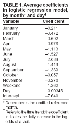 Return to top. Figure 1 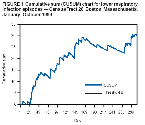 Return to top. Table 2 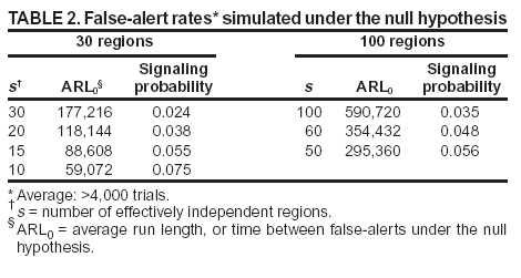 Return to top. Figure 2  Return to top. Figure 3 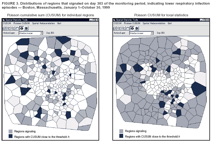 Return to top.
All MMWR HTML versions of articles are electronic conversions from ASCII text into HTML. This conversion may have resulted in character translation or format errors in the HTML version. Users should not rely on this HTML document, but are referred to the electronic PDF version and/or the original MMWR paper copy for the official text, figures, and tables. An original paper copy of this issue can be obtained from the Superintendent of Documents, U.S. Government Printing Office (GPO), Washington, DC 20402-9371; telephone: (202) 512-1800. Contact GPO for current prices. **Questions or messages regarding errors in formatting should be addressed to mmwrq@cdc.gov.Page converted: 9/14/2004 |
|||||||||
This page last reviewed 9/14/2004
|