Appendix 1
Calculating and Visualizing Four Indicators of Alcohol Outlet Density using R
Introduction
This file is an appendix to the Measuring Alcohol Outlet Density: A Toolkit for State and Local Surveillance pdf icon[PDF – 22 MB]. It was written by Mike Dolan Fliss, PhD, MPS, MSW, Research Scientist, University of North Carolina, Injury Prevention Research Center. It demonstrates the calculation of the four indicators for measuring alcohol outlet density using R. This program is designed for introductory-level R users. More experienced R users may choose to modify the program to complete their analyses.
Resources
Demonstration Code
#............................. ####

#.............................
# LIBRARIES & CONSTANTS ####
#.............................
# install.packages("tidyverse") # Will need to install these 1 time, then can just library
library(tidyverse) # for data science
## -- Attaching packages --------------------------------------- tidyverse 1.3.1 --## v ggplot2 3.3.5 v purrr 0.3.4
## v tibble 3.1.3 v dplyr 1.0.7
## v tidyr 1.1.3 v stringr 1.4.0
## v readr 2.0.0 v forcats 0.5.1## -- Conflicts ------------------------------------------ tidyverse_conflicts() --
## x dplyr::filter() masks stats::filter()
## x dplyr::lag() masks stats::lag()library(sf) # for spatial work## Linking to GEOS 3.9.0, GDAL 3.2.1, PROJ 7.2.1library(readxl) # for reading Excel files
library(janitor) # for cleaning messy (human focused) names##
## Attaching package: 'janitor'## The following objects are masked from 'package:stats':
##
## chisq.test, fisher.testlibrary(tidycensus) # for easily getting population data, polygons
library(tidygeocoder) # for geocoding, when necessary
library(ggspatial) # for north arrows, distance bars on ggplot maps
options(tigris_use_cache = TRUE) # Try to cache tidycensus downloads if possible, saves time
ftinmile = 5280; ftinmeter = 3.2808399
state_abbr = "NC"
state_long = "North Carolina"
# Would typically set known best local projection here,
# but will do below in a more verbose way for new learners
# local_proj = "+proj=lcc +lat_1=36.1666 +lat_2=34.3333 +lat_0=33.75 +lon_0=-79 +x_0=609601.2192024384 +y_0=0 +datum=NAD83 +units=us-ft +no_defs"
# local_proj = 2264
#.........................
# > Discover & save spatial projections for analysis math ####
#.........................
# Find all spatial projections. Use a projection local to your area.
# See https://spatialreference.org/ref/epsg/ for details.
epsg_tbl = rgdal::make_EPSG() %>% as_tibble() %>% mutate_all(as.character)
suggested_projections = epsg_tbl %>% # May work for you...
filter(str_detect(note, "NAD83 ")) %>% filter(str_detect(note, "(ft)")) %>%
filter(!str_detect(note, "deprecated")) %>% filter(str_detect(note, state_long))
suggested_projections## # A tibble: 2 x 4
## code note prj4 prj_method
## <chr> <chr> <chr> <chr>
## 1 2264 NAD83 / North Carolina (ftUS) +proj=l~ Lambert C~
## 2 8768 NAD83 / North Carolina (ftUS) + NAVD88 height (ftUS) +proj=l~ (null)# For NC we'll choose 2264 - NAD83, NC (ft US). These can be constants in the future.
local_projection = 2264
# Long-Lat coord system often useful.
wgs84_coordsystem = 4326
#.........................
# ^ See for primer:
# https://gis.stackexchange.com/questions/149749/is-wgs84-a-coordinate-system-or-projection-system
#......................... ####
#.####
#......................... ####
# GATHER POP DATA & POLYGONS ####
#.........................
# Your API key here. Or hard code.
# census_api_key("<INSERT YOUR API KEY HERE>", install = TRUE, overwrite = T)
# Get an api key here: https://api.census.gov/data/key_signup.html
# > Create helper table of census variables ####
# Can be done in excel/csv. See load_variables() for more.
census_data_vars = tribble(
~censuscodes, ~fieldname,
"B03002_001", "pop_tot", # All we will use in this simple analysis
"B03002_003", "pop_WNH", #.... but for considering disparities,
"B03002_004", "pop_Black", # you can calculate group-specific versions ...
"B03002_006", "pop_Asian",
"B03002_012", "pop_Hisp",
"B19013_001", "med_income", #... or track other interesting variables
)
# > Get counties from census API ####
# Can also get other geographies similarly, like tracts
county_acs = tidycensus::get_acs(geography = "county", survey="acs5",
geometry = T, state = state_abbr,
year=2019, variables = census_data_vars$censuscodes,
key=Sys.getenv("CENSUS_API_KEY"), output = "wide")## Getting data from the 2015-2019 5-year ACScounty_acs = county_acs %>% st_transform(local_projection) # Project right away
county_acs = county_acs %>% select(-matches("M$")) # Drop margins of error
# ^ Note that if you have different spatial levels (e.g., tracts, BGs)
# you can rbind() them together and calculate all at once.
# Create short names
county_acs$name_sm = county_acs$NAME %>% str_replace(" County,(.)*$", "")
# rename columns for convenience
name_index = census_data_vars$censuscodes %>% paste0("E") %>% match(names(county_acs))
names(county_acs)[name_index] = census_data_vars$fieldname
county_acs %>% head(3) # Take a look## Simple feature collection with 3 features and 9 fields
## Geometry type: MULTIPOLYGON
## Dimension: XY
## Bounding box: xmin: 406818.5 ymin: 488143.8 xmax: 1648058 ymax: 1028764
## Projected CRS: NAD83 / North Carolina (ftUS)
## GEOID NAME pop_tot pop_WNH pop_Black pop_Asian
## 1 37039 Cherokee County, North Carolina 27969 25450 348 203
## 2 37159 Rowan County, North Carolina 140296 101067 22033 1216
## 3 37171 Surry County, North Carolina 71971 60359 2581 409
## pop_Hisp med_income geometry name_sm
## 1 881 41438 MULTIPOLYGON (((408779.4 50... Cherokee
## 2 12381 49842 MULTIPOLYGON (((1474004 704... Rowan
## 3 7632 43597 MULTIPOLYGON (((1419518 989... Surry#.....................
# > Get block groups for distance-based measures ####
# (Takes a minute or so)
bg_acs = tidycensus::get_acs(geography = "block group", survey="acs5",
geometry = T, state = state_abbr,
year=2018, variables = census_data_vars$censuscodes,
key=Sys.getenv("CENSUS_API_KEY"), output = "wide")## Getting data from the 2014-2018 5-year ACSbg_acs = bg_acs %>% st_transform(local_projection) # Project right away
# Same as above, drop MOE and rename columns
bg_acs = bg_acs %>% select(-matches("M$")) # Drop MOE
names(bg_acs)[census_data_vars$censuscodes %>% paste0("E") %>% match(names(bg_acs))] = census_data_vars$fieldname
# Quick checks - drop empty geometries
broken_rows = st_is_empty(bg_acs)
bg_acs = bg_acs %>% filter(!broken_rows)
bg_acs = bg_acs[county_acs,] # spatially subset - require bgs to intersect county_acs
bg_acs %>% head(3) # Take a look## Simple feature collection with 3 features and 8 fields
## Geometry type: MULTIPOLYGON
## Dimension: XY
## Bounding box: xmin: 883178.2 ymin: 50425.64 xmax: 2175289 ymax: 629183.1
## Projected CRS: NAD83 / North Carolina (ftUS)
## GEOID
## 1 370190205123
## 2 371759603005
## 3 371190062091
## NAME pop_tot
## 1 Block Group 3, Census Tract 205.12, Brunswick County, North Carolina 284
## 2 Block Group 5, Census Tract 9603, Transylvania County, North Carolina 478
## 3 Block Group 1, Census Tract 62.09, Mecklenburg County, North Carolina 864
## pop_WNH pop_Black pop_Asian pop_Hisp med_income
## 1 283 0 0 1 78250
## 2 451 24 0 0 30313
## 3 721 73 10 60 53977
## geometry
## 1 MULTIPOLYGON (((2169994 536...
## 2 MULTIPOLYGON (((883178.2 55...
## 3 MULTIPOLYGON (((1437640 624...#..................... ####
#.####
#..................... ####
# PREPARE OUTLET DATA ####
#.....................
# Outlet data structure is highly specific to each jurisdiction. For North Carolina,
# a state with state-controlled license structure, the data is received in two parts -
# an excel file with multiple tables and a separate file of state-controlled ABC liquor
# stores. We'll need to combine these to accurately calculate outlet density. A helper
# table (made by public health) helps to code certain license types for study inclusion
# and license type.
# > Read License table ####
license_tbl = readxl::read_excel("data/NC/original data/Retail Establishments 2019_08_15.xlsx", col_types = "text") %>%
janitor::clean_names() %>% # Messy names. Let's clean right away w/ janitor
mutate(longitude = longitude %>% as.numeric, latitude = latitude %>% as.numeric)
license_tbl %>% head(3) %>% as.data.frame## file_number_temp_permit_number trade_name
## 1 00280201MB Club Eclipse
## 2 T00276738 Kings Food Mart 2
## 3 00255798AJ-999 Moe and D's Restaurant and Grill
## corp_name address city
## 1 Timothy Watlington Enterprises LLC 508 Teague Street Greensboro
## 2 Bansal LLC 3007 Hickory Grove Road Gastonia
## 3 Moe and D's Restaurant and Grill LLC 123 South Church Street Rocky Mount
## state zip county status mailing_address mailing_city
## 1 NC 27406 Guilford Pending-Temporary PO Box 853 Greensboro
## 2 NC 28056 Gaston Pending-Temporary 2416 Arden Gate Lane Charlotte
## 3 NC 27804 Nash Active <NA> <NA>
## mailing_state mailing_zip phone fax permit_number_temp_permit_number
## 1 NC 27402 3363838861 <NA> 00280201MB
## 2 NC 28262 <NA> <NA> T00276738
## 3 <NA> <NA> 2529773000 <NA> 00255798AJ
## longitude latitude
## 1 -79.78410 36.07426
## 2 -80.75346 35.34643
## 3 -77.79734 35.94162# Exploratory analysis
license_tbl %>% count(status) # May want to write this out to a csv.## # A tibble: 2 x 2
## status n
## <chr> <int>
## 1 Active 54362
## 2 Pending-Temporary 975# Filter to active permits
license_tbl = license_tbl %>% filter(status == "Active")
# NOTE: ^ Very simple method using their "active" status.
# May need to do work with active / expired dates
# Extract permit code for use
license_tbl$permit_code = license_tbl$permit_number_temp_permit_number %>% str_extract("[A-Z]+")
license_tbl %>% count(permit_code) %>% arrange(desc(n))## # A tibble: 42 x 2
## permit_code n
## <chr> <int>
## 1 AJ 9321
## 2 AL 8172
## 3 AK 8057
## 4 AM 7341
## 5 MB 6194
## 6 AO 4136
## 7 AN 3157
## 8 CE 1099
## 9 DF 950
## 10 A 858
## # ... with 32 more rows# Acknowledge missingness - # very complete data
license_tbl %>%
count(missing_lat = is.na(latitude)) %>%
mutate(pct_missing_lat = missing_lat / sum(missing_lat)*100) ## # A tibble: 2 x 3
## missing_lat n pct_missing_lat
## <lgl> <int> <dbl>
## 1 FALSE 53466 0
## 2 TRUE 896 100# Read permit type classifications
# (...to determine which to keep. Made by public health in collab w/ ABC)
permit_types = read_excel("data/NC/original data/NC_permit_type_classifier_2017.xlsx")
# From https://abc.nc.gov/Permit/Types
# Create a flag if the permit type we made is "known"
license_tbl = license_tbl %>% mutate(known_permit_type = permit_code %in% permit_types$permit_code)
# Check if any are uncategorized.
license_tbl %>%
count(permit_code, known_permit_type) %>%
filter(!known_permit_type)## # A tibble: 21 x 3
## permit_code known_permit_type n
## <chr> <lgl> <int>
## 1 A FALSE 858
## 2 B FALSE 645
## 3 BW FALSE 3
## 4 C FALSE 730
## 5 CP FALSE 450
## 6 D FALSE 635
## 7 E FALSE 549
## 8 F FALSE 554
## 9 G FALSE 3
## 10 GC FALSE 19
## # ... with 11 more rows# Some are unknown. Will eventually filter,
# but may need to talk with partners at ABC to refresh table
# Left join to our study inclusion table, and further filter
license_tbl = license_tbl %>%
left_join(permit_types %>% select(permit_code, permit_description, study_include, permit_group1)) %>%
filter(study_include == "Yes" & !(is.na(study_include))) ## Joining, by = "permit_code"# ^ Just keep know permit types with retail relevance
# > Collapse license table into outlet table ####
license_tbl %>% count(permit_group1)## # A tibble: 2 x 2
## permit_group1 n
## <chr> <int>
## 1 Off 19535
## 2 On 23041licensed_outlet_tbl = license_tbl %>%
count(trade_name, corp_name, address, city, state, longitude, latitude, permit_group1) %>%
group_by(trade_name, corp_name, address, city, state, longitude, latitude) %>%
summarize(n_premise_types = n(), n_licenses = sum(n),
permit_type = case_when("On" %in% permit_group1 ~ "On",
"Off" %in% permit_group1 ~ "Off",
TRUE ~ NA_character_))## `summarise()` has grouped output by 'trade_name', 'corp_name', 'address', 'city', 'state', 'longitude'. You can override using the `.groups` argument.# Acknowledge multi-premises types
licensed_outlet_tbl %>% filter(n_premise_types==2)## # A tibble: 1,282 x 10
## # Groups: trade_name, corp_name, address, city, state, longitude [1,282]
## trade_name corp_name address city state longitude latitude n_premise_types
## <chr> <chr> <chr> <chr> <chr> <dbl> <dbl> <int>
## 1 201 Central Harris Te~ 5939 W~ Wesl~ NC -80.7 35.0 2
## 2 20th Stree~ 20th Stre~ 2000 B~ More~ NC -76.7 34.7 2
## 3 220 Exxon Panch Par~ 1701 U~ Stok~ NC -79.9 36.3 2
## 4 421 Market~ Coulter M~ 1438 E~ Kern~ NC -80.0 36.1 2
## 5 427 Conven~ <NA> 1461 O~ Gree~ NC -77.4 35.6 2
## 6 580 Craft ~ 580 Craft~ 354 Ea~ Pitt~ NC -79.2 35.7 2
## 7 6 Twelve C~ Swami Sri~ 2109-1~ Rale~ NC -78.7 35.8 2
## 8 67 Gas For~ Samguru I~ 7915 R~ Pfaf~ NC -80.4 36.2 2
## 9 70 West Ma~ 70 West M~ 4401 A~ More~ NC -76.8 34.7 2
## 10 A'Nets Kat~ A'Nets Ka~ 2009 V~ Knig~ NC -78.5 35.8 2
## # ... with 1,272 more rows, and 2 more variables: n_licenses <int>,
## # permit_type <chr># Example : a Harris Teeter in Union, NC has both
# on and off-premise license types (file number: Q11307-752)
# > Add rows of ABC store data ####
# read supplemental state ABC stores to tack on....
abc_store_tbl = readxl::read_excel("data/NC/original data/ABC Store Information 08-15-2019_wheader.xlsx")
abc_store_tbl %>% head(3)## # A tibble: 3 x 9
## name street_address city state zip hours phone long lat
## <chr> <chr> <chr> <chr> <chr> <chr> <chr> <chr> <chr>
## 1 Alamance ~ 603 W Harden St~ Graham NC 27253 Mon-Sa~ 336-22~ -79.40~ 36.069~
## 2 Alamance ~ 1940 N Mebane St Burli~ NC 27215 Mon-Sa~ 336-22~ -79.45~ 36.073~
## 3 Alamance ~ 3012 S Church St Burli~ NC 27215 Mon-Sa~ 336-58~ -79.49~ 36.080~# Recode to look similar to licensed_outlet_tbl
abc_store_tbl = abc_store_tbl %>%
rename(trade_name = name, address = street_address, longitude = long, latitude = lat) %>%
mutate(latitude = if_else(latitude != "NULL", latitude, NA_character_), # Be explicit about NULL->NA rather than implicit coercion
longitude = if_else(longitude != "NULL", longitude, NA_character_), ) %>%
mutate(latitude = latitude %>% as.numeric, longitude = longitude %>% as.numeric) %>%
mutate(corp_name = "State ABC", n_premise_types = 1, n_licenses = 1, permit_type = "Off")
# Combine licensed outlets and ABC stores
licensed_outlet_tbl = licensed_outlet_tbl %>%
bind_rows(abc_store_tbl)
# > Example geocoding: ABC stores missing lat-long data ####
licensed_outlet_tbl = licensed_outlet_tbl %>%
mutate(full_addr = paste(address, city, state, zip, sep = ", "))
# For demonstration purposes let's geocode ABC stores missing geocodes
geocode_tbl = licensed_outlet_tbl %>%
filter(corp_name == "State ABC") %>%
filter(longitude %>% is.na)
geocode_tbl## # A tibble: 14 x 14
## # Groups: trade_name, corp_name, address, city, state, longitude [14]
## trade_name corp_name address city state longitude latitude n_premise_types
## <chr> <chr> <chr> <chr> <chr> <dbl> <dbl> <dbl>
## 1 Belmont AB~ State ABC 6425L W~ Belm~ NC NA NA 1
## 2 Concord AB~ State ABC 2940 De~ Conc~ NC NA NA 1
## 3 Hoke Count~ State ABC 235 Fla~ Raef~ NC NA NA 1
## 4 Johnston C~ State ABC 12524 N~ Bens~ NC NA NA 1
## 5 Mecklenbur~ State ABC 9920-A ~ Matt~ NC NA NA 1
## 6 Mecklenbur~ State ABC 6318 Pr~ Char~ NC NA NA 1
## 7 Moore Coun~ State ABC 3792 US~ Cart~ NC NA NA 1
## 8 Nash Count~ State ABC 125 Fal~ Rock~ NC NA NA 1
## 9 Troutman A~ State ABC 511 N M~ Trou~ NC NA NA 1
## 10 Wake Count~ State ABC 11360 C~ Wake~ NC NA NA 1
## 11 Wake Count~ State ABC 1505 Ba~ Wend~ NC NA NA 1
## 12 Walnut Cov~ State ABC 521 N, ~ Waln~ NC NA NA 1
## 13 Walnut Cov~ State ABC 521 N. ~ Waln~ NC NA NA 1
## 14 Warren Cou~ State ABC 101 Sti~ Litt~ NC NA NA 1
## # ... with 6 more variables: n_licenses <dbl>, permit_type <chr>, zip <chr>,
## # hours <chr>, phone <chr>, full_addr <chr># Some geocoders require registration of an API key before you can make calls.
# e.g., Sys.setenv("GEOCODIO_API_KEY" = "<YOUR.API.KEY.HERE>")
source("Code/set_author_api_keys.R") # keeping author key out of Toolkit code
geocode_results_tbl = geo_geocodio(geocode_tbl$full_addr, full_results = T)## Warning: `geo_geocodio()` was deprecated in tidygeocoder 1.0.3.
## Please use `geo()` instead.geocode_results_tbl$geocode_date = lubridate::today() # Best practice - time stamp your geocodes
geocode_results_tbl$geocode_method = "Geocodio" # ... or your chosen API geocoder
# Example results:
geocode_results_tbl %>% head(3)## # A tibble: 3 x 21
## address lat long formatted_address accuracy accuracy_type source
## <chr> <dbl> <dbl> <chr> <dbl> <chr> <chr>
## 1 6425L Wilkin~ 35.3 -81.0 6425 Wilkinson Bl~ 1 rooftop Gaston
## 2 2940 Derita ~ 35.4 -80.7 2940 Derita Rd, C~ 1 rooftop Cabarrus
## 3 235 Flagston~ 35.0 -79.2 Raeford, NC 28376 0.33 place TIGER/Lin~
## # ... with 14 more variables: address_components.number <chr>,
## # address_components.street <chr>, address_components.suffix <chr>,
## # address_components.formatted_street <chr>, address_components.city <chr>,
## # address_components.county <chr>, address_components.state <chr>,
## # address_components.zip <chr>, address_components.country <chr>,
## # address_components.secondaryunit <chr>,
## # address_components.secondarynumber <chr>, ...# Combine with original data
geocode_results_tbl = geocode_results_tbl %>% rename_with(~paste0("gc_", .x))
geocode_combo_tbl = geocode_tbl %>% bind_cols(geocode_results_tbl)
# Reintegrate geocodes with data
gc_licensed_outlet_tbl = licensed_outlet_tbl %>%
left_join(geocode_combo_tbl %>% ungroup %>% select(full_addr = gc_address, gc_lat, gc_long)) %>%
mutate(longitude = if_else(gc_long %>% is.na, longitude, gc_long),
latitude = if_else(gc_lat %>% is.na, latitude, gc_lat)) %>%
select(-gc_lat, -gc_long)## Joining, by = "full_addr"# > Convert to flat table to spatial sf object ####
outlets_sf = gc_licensed_outlet_tbl %>%
filter(!is.na(latitude), !is.na(longitude)) %>%
st_as_sf(coords = c("longitude", "latitude"), remove=F) %>% # x-y are long-lat...
st_set_crs(wgs84_coordsystem) %>% # ... in WGS84 assign coordinate ref system
st_transform(local_projection) # convert to local NAD83 projection
outlets_sf %>% st_geometry %>% plot(pch=".") # Note outlets outside of NC.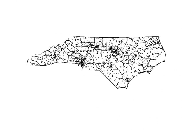
# ^ NOTE: Base R maps are FAST, good for quick visual tests. Other packages make prettier maps.

# > Subset to study area - otherwise may include far away / irrelevant outlets.
outlets_sf %>% st_intersects(county_acs) %>% map_int(length) %>% table
## .
## 0 1
## 830 17048outlets_sf = outlets_sf[county_acs,] # subset outlets to those in study zone
# > Quick maps ####
county_acs %>% st_geometry %>% plot
outlets_sf %>% st_geometry %>% plot(add=T, pch=".") # Quick double layer plot - looks better
# > Save our outlet work ####
outlets_sf %>% st_write("data/NC/study_outlets.shp", delete_layer = T)
## Warning in abbreviate_shapefile_names(obj): Field names abbreviated for ESRI
## Shapefile driver## Deleting layer `study_outlets' using driver `ESRI Shapefile'
## Writing layer `study_outlets' to data source
## `data/NC/study_outlets.shp' using driver `ESRI Shapefile'
## Writing 17048 features with 14 fields and geometry type Point.outlets_sf %>% st_set_geometry(NULL) %>% write_csv("data/NC/alcohol_outlets_demofile.csv")
outlets_sf %>% save(file = "data/NC/study_outlets.Rdata")
#................................
# Notes: Other descriptive statistics about your cleaned and spatial-ized data file
# may be useful. You might explore the tableone package (or others) to help with that.
#................................ ####
#.####
#.........................####
# SPATIAL ANALYSIS: COUNT-BASED MEASURES ####
#.........................####
county_AOD_sf = county_acs # let's work with a copy
# > (Helper) number of outlets ####
county_AOD_sf$n_outlets = st_intersects(county_AOD_sf, outlets_sf) %>% map_int(length)
# > (Helper) spatial area ####
county_AOD_sf$geo_area = st_area(county_AOD_sf) %>% units::set_units("mi^2") # area in sq mi
# ^ Could chase down details like land area, etc here.
# > (A1) number of outlets per 1,000 people ####
county_AOD_sf$n_v10k = county_AOD_sf$n_outlets / county_AOD_sf$pop_tot * 10000
# > (A2) number of outlets per square mile ####
county_AOD_sf$n_vsqmi = county_AOD_sf$n_outlets / county_AOD_sf$geo_area
# ^ NOTE tidyverse pipes and mutate()s could do this all at once. Breaking up for comments.
# > Quick choropleth maps ####
county_AOD_sf[,"n_v10k"] %>%
plot(main="Number of Outlets per 10,000 People")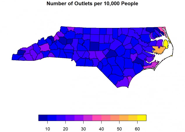
county_AOD_sf[,"n_vsqmi"] %>%
  plot(main="# outlets per square mile")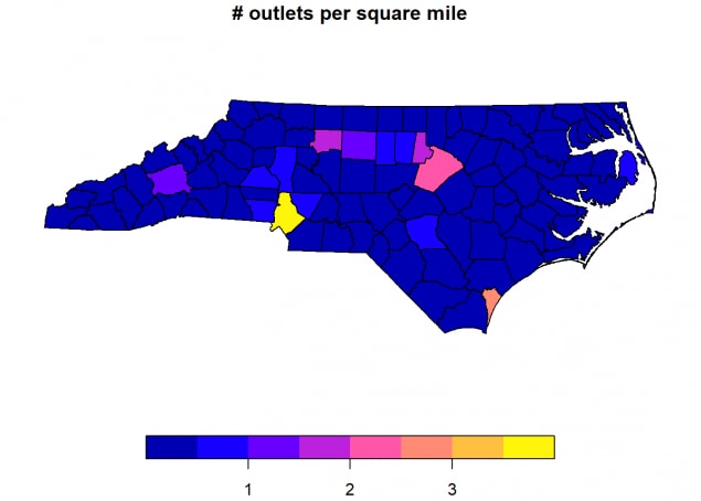
# Note not publication quality (consider export to QGIS), but good for testing

# Save for toolkit:
png(filename = "data/NC/outputs/map - simple - Number of Outlets per 10,000 People.png",
    pointsize=10, width=1400, height=960, res = 300) # <- Base plot methods
county_AOD_sf[,"n_v10k"] %>% plot(main="Number of Outlets per 10,000 People")
dev.off()
## png
## 2# Note small areas may have errors: 0 people/0 outlets -> NaN; N people / 0 outlets -> Inf -> NA
table(county_AOD_sf$n_v10k %>% is.na); table(county_AOD_sf$n_v10k %>% is.infinite)##
## FALSE
## 100##
## FALSE
## 100#.........................####
#.####
#.........................####
# SPATIAL ANALYSIS: DISTANCE-BASED MEASURES ####
#.........................####
# > (Helper calc) Pre-calculations for B1 ####
# pop centroid to outlet matrix
pop_distance_data = bg_acs %>% st_point_on_surface %>% # distance between pop centroids...
st_distance(outlets_sf) %>% units::set_units("mi") # ... and alcohol outlets in miles## Warning in st_point_on_surface.sf(.): st_point_on_surface assumes attributes are
## constant over geometries of xdim(pop_distance_data) # rows are BGs, cols are outlets## [1] 6137 17048pop_distance_data[1:5,1:5] # Skim the "corner" of the large matrix to see what we have## Units: [mi]
## [,1] [,2] [,3] [,4] [,5]
## [1,] 164.35910 194.39798 37.00390 218.99485 155.59135
## [2,] 190.88690 82.72241 281.77707 75.34935 114.32813
## [3,] 88.65607 23.19617 187.78005 42.97286 25.12846
## [4,] 39.18704 78.62536 185.16606 80.59686 76.99294
## [5,] 104.78746 191.46762 76.61705 207.93652 160.09189# Note this can take a minute or two. Check the tictoc package for easy timers
# pop centroid to min distance (start)
bg_acs$d_min = pop_distance_data %>% apply(MARGIN = 1, min, na.rm=T)
# bg_acs$d_min = distance_data %>% array_tree(margin=1) %>% map_dbl(min, na.rm=T)
# ^ purrr alternative
# > (B1) Distance from people to nearest outlet (V1) ####
# Variation #1: Tabular assignment of pop points to counties, weighted-avg calcs
d_popmin_tbl = bg_acs %>%
mutate(intersect_group = substr(GEOID, 1, 5)) %>%
group_by(intersect_group) %>%
summarize(d_popmin = sum(pop_tot * d_min) / sum(pop_tot, na.rm=T)) %>%
st_set_geometry(NULL) %>%
rename(GEOID = intersect_group)
d_popmin_tbl## # A tibble: 100 x 2
## GEOID d_popmin
## * <chr> <dbl>
## 1 37001 0.905
## 2 37003 2.18
## 3 37005 2.04
## 4 37007 3.21
## 5 37009 3.29
## 6 37011 2.76
## 7 37013 1.82
## 8 37015 3.21
## 9 37017 4.00
## 10 37019 1.26
## # ... with 90 more rows# Note that variation works BGs exactly nest in tracts which nest in counties.
# Variation #2 is more robust, and works for when pop points
# do not nest perfectly in the area of interest, e.g., districts or special areas
county_AOD_sf$d_popmin = d_popmin_tbl$d_popmin[match(county_AOD_sf$GEOID, d_popmin_tbl$GEOID)]
# county_AOD_sf = county_AOD_sf %>% left_join(d_popmin_tbl)
# ^ left join also works. Top version is repeatable.
# > (B1) Distance from people to nearest outlet (V2) ####
# TODO
# ----Consider a more robust (county+tract) method, like purrr ####
# Variation #2: Spatial assignment of pop points to counties, weighted-avg calcs
pop_intersection_list = bg_acs %>%
st_point_on_surface %>%
st_intersects(county_AOD_sf)## Warning in st_point_on_surface.sf(.): st_point_on_surface assumes attributes are
## constant over geometries of x# ^ Note also that st_centroid()s can be outside polygon;
# st_point_on_surface guarantees inside
# See https://geocompr.robinlovelace.net/geometric-operations.html#centroids for details
# Assign block groups (by point) to counties.
bg_acs$intersect_group = county_acs$GEOID[pop_intersection_list %>% unlist]
# Calculated pop weighted average of distance
d_popmin_tbl2 = bg_acs %>%
group_by(intersect_group) %>%
summarize(d_popmin = sum(pop_tot * d_min) / sum(pop_tot, na.rm=T)) %>%
st_set_geometry(NULL) %>%
rename(GEOID = intersect_group)
d_popmin_tbl2## # A tibble: 100 x 2
## GEOID d_popmin
## * <chr> <dbl>
## 1 37001 0.905
## 2 37003 2.18
## 3 37005 2.04
## 4 37007 3.21
## 5 37009 3.29
## 6 37011 2.76
## 7 37013 1.82
## 8 37015 3.21
## 9 37017 4.00
## 10 37019 1.26
## # ... with 90 more rowsidentical(d_popmin_tbl, d_popmin_tbl2)## [1] TRUE#................................
# > (Helper calc) Pre-calculations for B2 ####
# outlet to outlet matrix
outlet_distance_data = outlets_sf %>% # distance between outlets...
st_distance(outlets_sf) %>% units::set_units("mi") # ... and outlets in miles
dim(outlet_distance_data) # rows are BGs, cols are outlets## [1] 17048 17048diag(outlet_distance_data) = NA # Convert distance to self to NA
outlet_distance_data[1:5,1:5] # Skim the "corner" of the large matrix ## Units: [mi]
## [,1] [,2] [,3] [,4] [,5]
## [1,] NA 110.01887 157.0850 117.18455 95.81078
## [2,] 110.01887 NA 208.0698 26.48890 38.81533
## [3,] 157.08496 208.06979 NA 230.73662 170.11212
## [4,] 117.18455 26.48890 230.7366 NA 64.13631
## [5,] 95.81078 38.81533 170.1121 64.13631 NA# Note this can take a minute or two. Check the tictoc package for easy timers
# pop centroid to min distance (start)
outlets_sf$d_min = outlet_distance_data %>% apply(MARGIN = 1, min, na.rm=T)
# bg_acs$d_min = distance_data %>% array_tree(margin=1) %>% map_dbl(min, na.rm=T)
# ^ purrr alternative
# > (B2) Distance from outlet to next nearest outlet ####
outlet_intersection_list = outlets_sf %>% st_intersects(county_AOD_sf)
outlet_intersection_list %>% map_int(length) %>% table # Each outlet intersects 1 area.## .
## 1
## 17048# Assign block groups (by point) to counties.
outlets_sf$intersect_group = county_acs$GEOID[outlet_intersection_list %>% unlist]
# Calculated pop weighted average of distance
d_outmin_tbl = outlets_sf %>%
group_by(intersect_group) %>%
summarize(d_outmin = mean(d_min, na.rm=T)) %>%
st_set_geometry(NULL) %>%
rename(GEOID = intersect_group)
d_outmin_tbl## # A tibble: 100 x 2
## GEOID d_outmin
## * <chr> <dbl>
## 1 37001 0.276
## 2 37003 0.574
## 3 37005 0.997
## 4 37007 0.361
## 5 37009 0.433
## 6 37011 0.288
## 7 37013 0.684
## 8 37015 1.10
## 9 37017 0.401
## 10 37019 0.342
## # ... with 90 more rowscounty_AOD_sf$d_outmin = d_outmin_tbl$d_outmin[match(county_AOD_sf$GEOID, d_outmin_tbl$GEOID)]
# county_AOD_sf = county_AOD_sf %>% left_join(d_outmin_tbl)
# ^ left join also works. Top version is repeatable.
# > Quick choropleth maps ####
county_AOD_sf[,"d_popmin"] %>%
plot(main="Distance from person to their nearest outlet (mi)")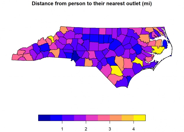
county_AOD_sf[,"d_outmin"] %>%
  plot(main="Distance from outlet to their nearest neighbor outlet (mi)")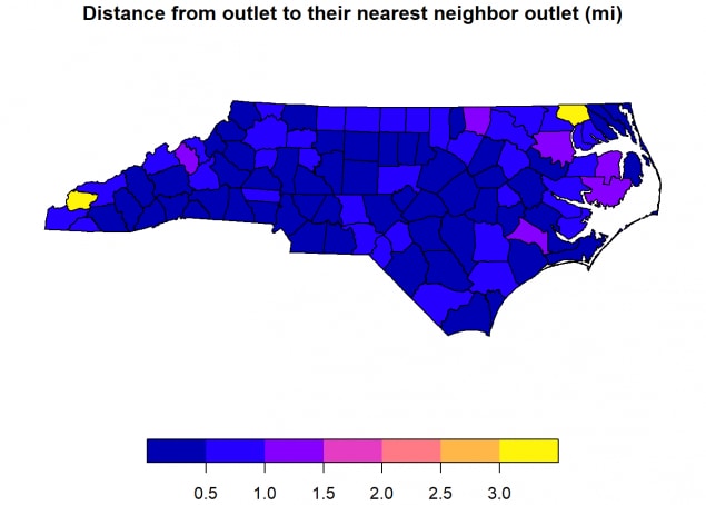
#................................ ####

#.####

#................................ ####
# Analysis complete. Write summary file: ####
#................................
county_AOD_sf %>% st_write("data/NC/outputs/county_AOD_sf.shp", delete_layer = T)
## Deleting layer `county_AOD_sf' using driver `ESRI Shapefile'
## Writing layer `county_AOD_sf' to data source
## `data/NC/outputs/county_AOD_sf.shp' using driver `ESRI Shapefile'
## Writing 100 features with 15 fields and geometry type Multi Polygon.# ^ Note that shapefiles (not always the ideal output type) are restricted to short variable names.
# Other spatial object alternatives work too, like geojsons.
county_AOD_sf %>% save(file = "data/NC/county_AOD_sf.Rdata")
#................................ ####
#.####
#................................ ####
# Step 7: Viz ####
#................................ ####
county_AOD_sf %>% names## [1] "GEOID" "NAME" "pop_tot" "pop_WNH" "pop_Black"
## [6] "pop_Asian" "pop_Hisp" "med_income" "geometry" "name_sm"
## [11] "n_outlets" "geo_area" "n_v10k" "n_vsqmi" "d_popmin"
## [16] "d_outmin"county_AOD_sf[, c("n_v10k", "n_vsqmi", "d_popmin", "d_outmin")] %>% plot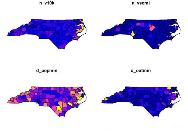
# Nicer ggplot example, w/ saving
graph_title = "Number of Alcohol Outlets per 10,000 People"
ggplot()+
  geom_sf(data=county_AOD_sf, aes(fill=n_v10k))+
  geom_sf(data=outlets_sf, pch=".")+
  scale_fill_distiller(type="div")+
  theme_void()+
  labs(title=graph_title,
       subtitle="Rate per 2019 county resident population",
       fill = "# outlets \n per 10k",
       caption=paste0("Data from 2019, including ",
                      prettyNum(outlets_sf %>% nrow, big.mark = ","),
                      " alcohol outlets"))+
  annotation_north_arrow(height = unit(.5, "cm"), width = unit(0.5, "cm"),
                         style = north_arrow_minimal(), location = "rl")+
  annotation_scale(location = "bl", unit_category = "imperial")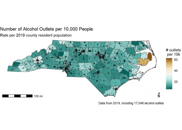
ggsave(paste0("data/NC/outputs/map - robust - ", graph_title, ".png"), dpi = 300)## Saving 7 x 5 in image# Note setting caption programmatically with number of outlets.
# This is best practice - try not to hard code things.
# Also look at tmap, plotly for interactive maps, etc.
beepr::beep() # Oven timer sound to let you know analysis is complete.
Page last reviewed: October 28, 2021
