Research Methods Bivariate Method for Spatio-Temporal Syndromic Surveillance

Persons using assistive technology might not be able to fully access information in this file. For assistance, please send e-mail to: mmwrq@cdc.gov. Type 508 Accommodation and the title of the report in the subject line of e-mail.

Research Methods
Bivariate Method for Spatio-Temporal Syndromic Surveillance

Al Ozonoff, L. Forsberg, M. Bonetti, M. Pagano
Harvard School of Public Health, Boston, Massachusetts

Corresponding author: Marcello Pagano, Department of Biostatistics, Harvard School of Public Health, 655 Huntington Avenue, Boston, MA 02115. Telephone: 617-432-4911; Fax: 617-739-1781; E-mail: pagano@hsph.harvard.edu.

Abstract

Introduction: Statistical analysis of syndromic data has typically focused on univariate test statistics for spatial, temporal, or spatio-temporal surveillance. However, this approach does not take full advantage of the information available in the data.

Objectives: A bivariate method is proposed that uses both temporal and spatial data information.

Methods: Using upper respiratory syndromic data from an eastern Massachusetts health-care provider, this paper illustrates a bivariate method and examines the power of this method to detect simulated clusters.

Conclusions: Syndromic surveillance systems should use all available information, including both spatial and temporal information.

Introduction

In 2002, CDC advised health departments to seek routinely collected electronic data as part of early warning systems for biologic terrorism (1). The potential cost-effectiveness of such systems might explain why certain major metropolitan areas (e.g., Boston and New York) are beginning to implement CDC's recommendation (2,3). The primary concern of a biosurveillance system is to analyze and interpret data as they are collected and then decide whether further investigation is required. This report proposes a statistical methodology needed to make such a system efficient and effective and focuses on how to use information about the number of patients affected and where they live to detect outbreaks or other deviations from the normal pattern of disease.

Two statistical concerns are fundamental to surveillance: 1) determining a reasonable definition of "normal" behavior, and 2) being vigilant for deviations from this normalcy. CDC's weekly surveillance for pneumonia and influenza mortality in 122 U.S. cities is one example of an attempt to put this into practice (see MMWR Weekly at http://www.cdc.gov/mmwr). In that model, historic data allow for time-series modeling of seasonal fluctuations in deaths; the model represents an attempt to define normalcy. Building on a sinusoidal model for the seasonal baseline, standard statistical methods (4) provide a confidence band outside of which mortality can be considered a deviation from the norm. Such a definition of normalcy is too stringent because deviations from normalcy occur almost every year; therefore, its usefulness for a surveillance system might be questionable. However, a too-lenient definition of normalcy might then never detect a deviation from normal.

Combining Univariate Statistics

Combining more than one test statistic from a single data source poses problems. In certain situations, multiple testing without an appropriate statistical adjustment leads to an inflation of the false-positive rate. However, such adjustments can be conservative and adversely affect the power of the tests.

One approach that avoids the multiple-testing problem involves investigating the joint distribution of the test statistics. As a result, the information encoded in each statistic is used, but the false-positive rate can still be carefully controlled. The bivariate methodology described in this paper is one example of combining univariate statistics. Although the concept generalizes easily to other settings, implementation of this methodology will necessarily differ, depending on the situation. The requirements and assumptions (as well as the strengths and weaknesses) of the particular univariate models and statistics used will affect the power and robustness of any implementation of this bivariate approach.

Data

Data for this study were obtained from a major health-care provider in eastern Massachusetts. As patients arrive for emergency care, their cases are geocoded (typically by using the patient's residential or billing address); this information is centralized electronically on a daily basis. For this study, a subset of the data was selected, consisting of upper respiratory infections (URIs) during January 1, 1996--October 30, 2000, for a period of 1,399 days. (For protection of confidentiality, the spatial data provided in this report were aggregated by census tract and white noise was added to the centroids of the tracts.) Thus, the data stream provides the temporal patterns of disease (i.e., the number of cases arriving each day), as well as the spatial patterns of disease (i.e., the locations of patients over time).

Using all available information should provide better detection power than using just the number of patients or only their locations. Thus, the proposal is to analyze the temporal series first, then the spatial series, and, finally, to conduct a joint analysis of the two.

Methods

Time-Series Modeling

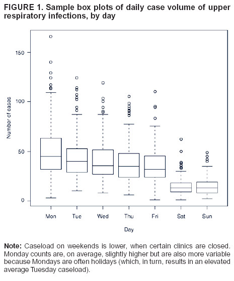
Time-series modeling is one approach for analyzing temporal data. Certain trends in the number of patients reporting daily with URIs make modeling challenging. One such trend is a seasonal effect, which can be modeled efficiently. Superimposed on the seasonal effect is a substantial daily effect, including a slight downward trend in the number of URIs from Monday through Friday, as well as a substantially higher variance from the start of the week to the end (Figure 1). Weekends and holidays must be analyzed separately because certain clinics and other locations are closed on those days, resulting in lower case volume and a different spatial distribution of patients. Health-care demand for weekends and holidays is often satisfied on Mondays or weekdays immediately after holidays, resulting in a higher case volume on those days.

For the time series N(t) of number of URIs to be accurately modeled, a sinusoidal baseline curve must first be fitted to account for seasonal variations. Each data point can then be considered as a residual departure from the baseline prediction. The residuals are then modeled to find a best predicted value of N(t). Because patient behavior varies by day of week, days are categorized as follows: 1) weekend days or holidays; 2) Mondays or days after holidays; and 3) all other weekdays. Seasonal and daily effects are incorporated into a linear model. The residuals from this mean function are autocorrelated; therefore, a third-order autoregressive component and a first-order moving average component (Autoregressive Moving Average [ARMA] [3,1] are used to model this autocorrelation. Thus, the final model is formulated as

where e(t) is the residual (observed or predicted value) at time t, and the β, γ are ARMA coefficients estimated from a standard statistical package. The standard deviation of the residuals is used as a measure of the model's goodness-of-fit. After inclusion of the ARMA terms, the standard deviation of the residuals was reduced from 0.732 to 0.321 (on the log scale), indicating that the ARMA series has a better fit than the simple sinusoid. Standard deviations for holidays and weekends, Mondays and days after holidays, and other weekdays are all comparable; however, these are measured on the log scale, and thus, the higher case volume on Mondays and days after holidays, together with greater variation on those days (Figure 1), reduces the model's predictive power for those days as compared with weekends and holidays, which have lower mean case counts.

The time series N(t) is an attempt to describe normal behavior. The residuals are distributed approximately normally with mean 0, and a nominal alpha level can be chosen on the basis of historic data, and any observation falling outside of a particular critical region can be considered worthy of investigation.

Spatial Statistic

Temporal analysis provides only one perspective, albeit a classic one, of the information in the surveillance data (i.e., the number of patients) The geocoded portion of the data set (i.e., the location of the patients) provides a second perspective. Other researchers have used spatial analytic approaches (2,3,5) on the assumption that terrorist attacks might produce a pattern of disease with a distinctive spatial signature (6).

Multiple spatial statistics have been designed to detect distinctive spatial patterns (7,8). Because the particular disease pattern that a terrorist attack might produce remains unknown, a statistic should be sufficiently flexible to detect multiple distortions from normalcy without requiring a priori knowledge of how such a distortion might appear. For this analysis, simple application of the M-statistic (9), which is based on the distribution of distances between patients, was chosen. To compute the M statistic for detection of outbreaks, all pairwise distances between locations of patients arriving for care each day are calculated. An empirical cumulative distribution function (ECDF) of these distances can then be compared with the historically determined distribution of distances to yield a test statistic, M. Asymptotic properties of the M statistic (9) or empirical simulation allow for a nominal alpha level to determine substantial deviations from the norm.

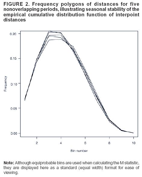
Fundamental to use of the M statistic is the remarkable stationarity of the distribution of distances over time. The frequency polygon of distances, derived from the ECDF, for five randomly chosen, nonoverlapping 30-day periods distributed across seasons and throughout the approximate 4-year study period, is illustrated (Figure 2). The ECDF is sufficiently stable from season to season and year to year to establish a definition of normalcy.

Daily geocoded data enables 1) calculation of the ECDF

(where F(D) denotes the cumulative distribution function of interpoint distances determined from historic data) for each day's disease cases, and 2) calculation of a test statistic measuring the departure from F(D). To avoid complexities, the daily case load is used to calculate distances between patients; typically, memory can be incorporated into the system by extending a temporal window within which to calculate distances. This extension would be especially important when dealing with a contagious ailment that has an incubation distribution. To facilitate calculation of the statistic, all of the interpoint distances are placed into 10 bins that are equiprobable under the distribution F(D), and a Mahalanobis-like distance is calculated as

where o is the 10-dimensional vector of observed proportions of distances in each bin; e is the vector of expected proportions (equal to [0.1, … , 0.1]) under the null distribution; and S is an estimator of the variance-covariance matrix Σ of the bin proportions calculated under the null. S is calculated from the historic data and a generalized inverse S^-- is used because S is not of full rank.

Because the distribution of distances between patients is stationary, an alert based on M can be instituted so that large values of M generate the alert; exactly how large these values must be is determined by the desired false-positive rate. The null distribution of M is determined by the null distribution of the distances; however, asymptotically, NM has a χ² distribution with degrees of freedom equal to the rank of the covariance matrix Σ ˉ Σ (where NM refers to the product of the test statistic M(t) and number of cases N at a time t). Thus, the distribution of NM is asymptotically independent of the number of cases used to calculate the statistic. As the degrees of freedom increase, the log of a χ² random variable approximates a normal distribution, and experience has confirmed that the values log(NM) give a close normal approximation. More importantly, this demonstrates that the random variables NM and N are approximately independent for large N (i.e., N >40). Thus, the temporal information and spatial information are orthogonal (for large N).This substantiates combining the two to produce an even more powerful statistic, as discussed in the following section.

Bivariate Test Statistic

Use of a bivariate test statistic, composed of the two statistics described previously, is proposed to increase the power of outbreak detection. N(t) permits calculation of a residual value for the number of cases arriving, on the basis of the time-series prediction for that day, with residuals that are approximately normal. Log(NM) expresses the deviation of the spatial distribution of cases from normalcy, and this statistic is approximately normal as well. Standard techniques from multivariate analysis can be used to construct an elliptical rejection region for a bivariate normal population at prespecified alpha level (false-positive rate) that can be used to detect deviations from normalcy. However, this might not offer particular protection against the alternative of interest (i.e., an outbreak resulting from release of a biologic agent).

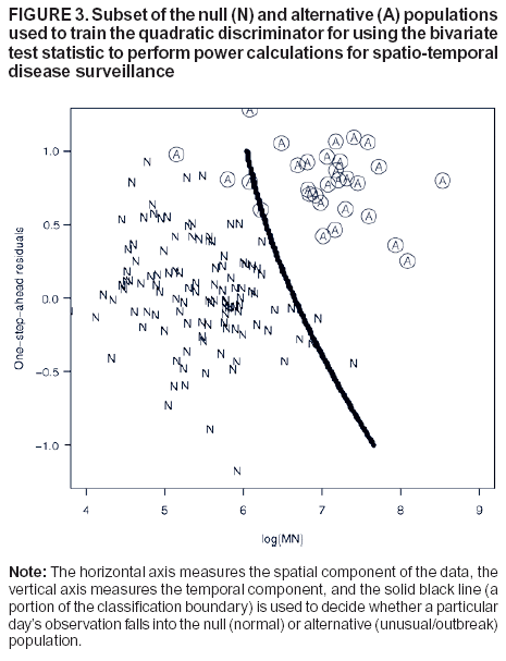
As another approach, potential biologic attacks can be modeled to simulate bivariate values in the event of an attack; in this case, an optimal discriminator (the quadratic classification rule) exists between two bivariate normal populations: 1) the bivariate distribution under the null, and 2) the modeled bivariate distribution under the alternative of a biologic attack (10). The classification rule is a quadratic form that, given log(NM) and the one-step-ahead time-series residuals, assigns one day's observations to either the null or alternative population. This rule minimizes the expected error of misclassification. The false-positive rate can be controlled by shifting the quadratic boundary appropriately, as determined through simulation or resampling of the historic record. A typical case of the null and alternative populations, together with the boundary of the discriminator, is illustrated (Figure 3).

Results

Because no biologic terrorism events occurred in eastern Massachusetts during the period of study, an outbreak simulation was necessary. To this end, for each of four locations, either six, nine, or 12 additional URIs were added to the existing data set. The range of 6--12 cases represents approximately 0.25--1.25 standard deviations of the original caseload, depending on the day of the week (mean daily case count is approximately 15 cases/day on weekends, 55 cases/day on Mondays, and 40 cases/day on other weekdays). The signal was dispersed across adjacent census tracts (i.e., adding six cases at a particular location amounted to choosing six nearby tracts and adding one case to each tract). (For brevity, such a simulated signal is called a cluster.) By using the statistics discussed previously, power was calculated on the basis of this simulated disease signal. Although other methods might have higher power to detect a concentrated cluster (e.g., six additional cases in one tract), they are less likely to perform as well when the signal is dispersed.

A simulated cluster was added to each of the 1,399 days of data, 1 day at a time, to assess how frequently different statistics might detect such a signal. Power calculations were performed separately for each of the three daily categories (weekend days or holidays, Mondays or days after holidays, and all other weekdays) because prediction and behavior differ within each of these categories. A detection threshold was set for each statistic on the basis of an alpha level of 0.05. For daily observations (as are illustrated here), this is equivalent to one false alert every 20 days. Power equals the ratio of detections to the total number of observations.

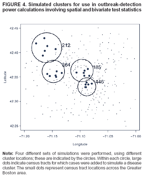
The four locations chosen for the simulation are in different geographic areas covered by the data. Previous simulations have demonstrated that power to detect a cluster might depend on the local geography and location of the signal source (11). This effect is confounded by the population distribution in the data available. Locations on the outskirts of the region covered tend to be more sparsely populated; hence, the signal is more widely dispersed. The census-tract locations in the study area, together with the four locations at which clusters were simulated, are illustrated (Figure 4). The cluster at location 446 corresponds to an area approximately circular with radius 0.5 miles; at locations 185 and 364 with radius 1 mile; and at location 212 with radius 1.5 miles. These radii reflect population densities.

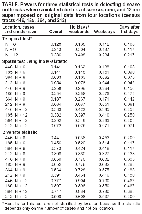
Power calculations for the three test statistics are provided (Table). Results for the univariate test statistic N based on time-series modeling are not stratified by location because the statistic depends only on the number of cases and not on locations. Power to detect an additional six, nine, or 12 cases added to the case counts of the final 399 days of data was then calculated by using the first 1,000 days to train the model (Table).

Next, a training sample was generated based on a modeled signal consisting of 12 cases near location 446, superimposed on each of the first 1,000 days of data. This permitted generation of two distinct bivariate normal populations of values, consisting of N(t) residuals together with log(NM) calculations, as a training sample. Next, for a simulated cluster in the final 399 days of data, the corresponding bivariate test statistic was calculated, and the quadratic classification rule was used to place each day's simulated cluster into the null (no signal) population or the alternative (signal present) population (Table). Power in this case equals the number of clusters classified in the alternative divided by the total number of observations.

Conclusions

The power of the univariate statistic N, which detects deviations from the predicted number of cases daily, illustrates the difficulties of time-series modeling for public health surveillance. The behavior of the time series N(t) is nonstationary, with differing variation according to season and day of the week. Rather than relying on a simple autoregression, detection results could be improved by considering a multivariate periodic autoregression (12). Meanwhile, the spatial statistic M has exhibited promise in other contexts to detect spatial deviations from the norm (3,9). Further research into the characteristics of this and other spatial statistics is needed, as different complementary spatial methods exist that can be used in conjunction with differing detection power.

Development of additional statistical methods and research into those methods are critical to the terrorism surveillance effort. Because routinely collected electronic data are often available to public health departments and researchers, efficient analysis of these data provides a low-cost method for surveillance. Although one cannot make any claims as to the robustness or generalizability of the bivariate method to other data sets or other univariate statistics, the power calculations provided here demonstrate that information on the number of cases as well as the spatial distribution of those cases can be used effectively in combination to improve the efficiency of surveillance systems.

This project was funded in part by grants from the National Institutes of Health (Grant no. RO1AI28076) and the National Library of Medicine (Grant no. RO1LM007677).

References

Use of trade names and commercial sources is for identification only and does not imply endorsement by the U.S. Department of Health and Human Services.

References to non-CDC sites on the Internet are provided as a service to MMWR readers and do not constitute or imply endorsement of these organizations or their programs by CDC or the U.S. Department of Health and Human Services. CDC is not responsible for the content of pages found at these sites. URL addresses listed in MMWR were current as of the date of publication.

Disclaimer All MMWR HTML versions of articles are electronic conversions from ASCII text into HTML. This conversion may have resulted in character translation or format errors in the HTML version. Users should not rely on this HTML document, but are referred to the electronic PDF version and/or the original MMWR paper copy for the official text, figures, and tables. An original paper copy of this issue can be obtained from the Superintendent of Documents, U.S. Government Printing Office (GPO), Washington, DC 20402-9371; telephone: (202) 512-1800. Contact GPO for current prices.